1. Introduction of self encoder
The idea of self Encoder is very simple. It is to convert an image into a code through Encoder, and then reconstruct the generated code into an image through Decoder, and then hope that the reconstructed image is closer to the original image.
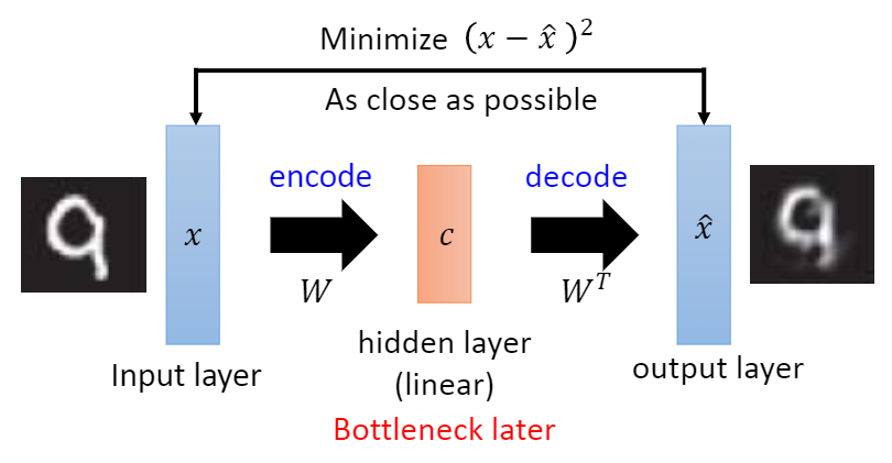
1) Traditional self encoder
The traditional self encoder is realized by neural network
The purpose of traditional self coder is to make the output and input as same as possible, which can be completed by learning two identity functions, but such transformation is meaningless, because we really care about the hidden layer expression rather than the actual output. Therefore, many improvement methods for self coder are to add certain constraints to the hidden layer expression, Force the hidden layer expression to be different from the input. If the model can reconstruct the input signal at this time, it shows that the hidden layer expression is enough to represent the input signal, and this hidden layer expression is the effective feature automatically learned by the model
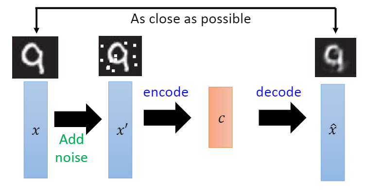
2) Noise reduction self encoder
A good expression should be able to capture the stable structure of the input signal, have certain robustness, and be useful for reconstructing the signal
The proposal of noise reduction self encoder is inspired by a phenomenon that human beings can still accurately recognize partially occluded or damaged images. Therefore, the main research goal of noise reduction self encoder is to express the robustness of hidden layer to locally damaged input signals. That is, if a model has sufficient robustness, Then the expression of locally damaged input on the hidden layer should be almost the same as that of clean input without damage, and the clean input signal can be reconstructed by using this hidden layer expression
Therefore, the noise reduction self encoder artificially adds some noise to the clean input signal, so that the clean signal is locally damaged and generates a damaged signal corresponding to it, and then sends the damaged signal to the traditional self encoder to reconstruct an output similar to the clean input as much as possible
3) Convolutional self encoder
The excellent performance of convolutional neural network directly promotes the generation of convolutional self encoder. Strictly speaking, convolutional self encoder belongs to a special case of traditional self encoder, which uses convolution layer and pooling layer to replace the original full connection layer. Traditional self encoder generally uses full connection layer, which has no impact on one-dimensional signal, For two-dimensional image or video signal, the full connection layer will lose spatial information. By using convolution operation, the convolution self encoder can well retain the spatial information of two-dimensional signal
The convolutional self encoder is very similar to the traditional self encoder. The main difference is that the convolutional self encoder linearly transforms the input signal by convolution, and its weight is shared, which is the same as that of convolutional neural network. Therefore, the reconstruction process is the linear combination of basic image blocks based on hidden coding
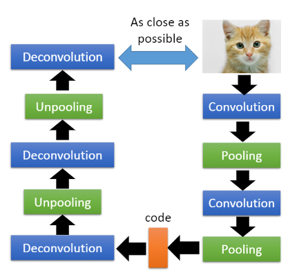
There may be some understanding problems with Unpooling and Deconvolution.
- Unpooling
We know that the pooling layer in convolution is to de average or de maximize the original local area to reduce the size. Usually, the scale size after pooling is one-half of the original size. Alternatively, pooling can also be understood as down sampling. Unpooling can be understood as upsampling.
One way to achieve this is to retain the memory of the previous pool, that is, to remember the region where the maximum value is selected, and then when the scale expands, retain the maximum value, and then fill 0 in other places, so as to increase the size.
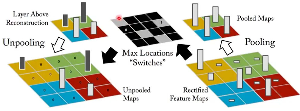
Another way is to as like as two peas in a single expansion area, instead of 0.
Effect after Unpooling:
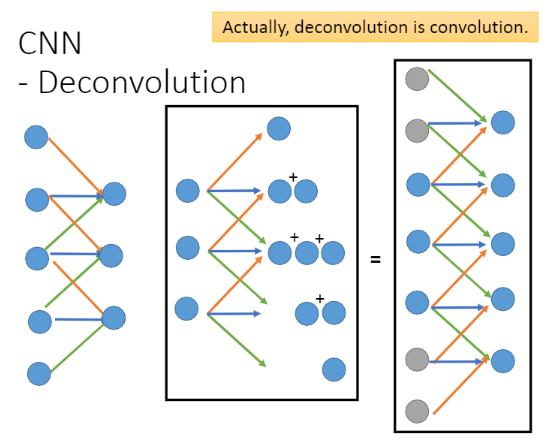
2. Deconvolution
In fact, Deconvolution is revolution, where revolution reduces the dimension through convolution, and Deconvolution can expand the dimension through padding. As shown in the following figure, revolution is the operation on the left, and Deconvolution is actually the operation on the right.
2. Application of self encoder
The hidden variable code obtained based on the dimensionality reduction of the self encoder can actually have some applications.
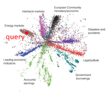
1) Text Retrieval
We can regard an article as a data distribution in a two-dimensional space. An article represents a point in the data distribution, so we can extract an article into a two-dimensional code through the self encoder.
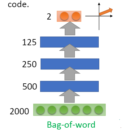
Then, according to the distribution of the two-dimensional code in the data space, we can retrieve its acquaintance with other articles, so as to realize classification or other operations.
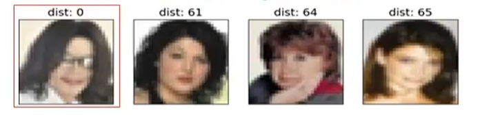
2) Familiar image search
In fact, we can also carry out image retrieval through the ability of self coding to find data distribution. The specific operation is that when we want to find some familiar images, if we use the familiarity between the pixels, that is, if we eliminate the distribution of pixels between the two images, the results are often not very good.
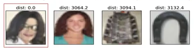
However, at this time, we can turn the image we need to find into a code through the encoder, and then retrieve it through this code. In other words, if the difference between the codes of the two images is relatively small, we can believe that it is possible to find the image we need, and the final result is often better than the result of finding the distribution between pixels. At least we know from the code in the encoder that we are looking for a portrait.
3) Pre training of model
We know that initialization is usually very important in the training of neural networks, so in fact, we can use self encoder to realize the operation of pre training.
When we conduct semi supervised learning, we usually have a lot of unlabeled data, and then only a small part of data with label. At this time, we can use these large amounts of unlabeled data to pre train the model.
We assume that the model structure is a fully connected neural network structure with three hidden layers. For the first hidden layer, we input an image, and then get a 1000 dimensional code through the hidden layer through the self encoder, which is actually the hidden layer of the second layer. Of course, it needs to be avoided at this time. When the code is higher than the dimension of the image, the network can directly retain the dimension information of the whole image intact. We need to pay attention to this. Then reconstruct the code into the original model through the Decoder. At this time, we can fix the parameters of the first hidden layer, because it has been trained.
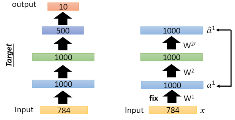
Similarly, we can train the second hidden layer, turn the second layer into a code, and the dimension of this code is the dimension of the third hidden layer, then reconstruct it, and then fix the parameters of the second hidden layer.
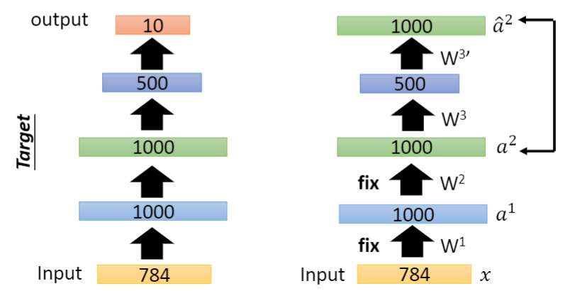
Similarly, for other hidden layers, the operation is similar. When the parameters of all network layers are reserved, the network has been pre trained. Now you only need to use a small amount of data with label to back propagate the network, and you can adjust the parameters slightly.
However, in fact, for the current network, it is generally possible to train without initialization, but this is due to the improvement of training technology. In the past, there was a large gap between non initialization and initialization.
3. Implementation of self encoder
Use pytoch framework
The dataset uses MNIST
Reference code
model.py
import torch
import torchvision
import torch.nn as nn

# Define self encoder structure
class Auto_Encoder(nn.Module):

    def __init__(self):

        super(Auto_Encoder, self).__init__()

        # Define encoder structure
        self.Encoder = nn.Sequential(
            nn.Linear(784, 256),
            nn.ReLU(),
            nn.Linear(256, 64),
            nn.ReLU(),
            nn.Linear(64, 20),
            nn.ReLU()
        )

        # Define decoder structure
        self.Decoder = nn.Sequential(
            nn.Linear(20, 64),
            nn.ReLU(),
            nn.Linear(64, 256),
            nn.ReLU(),
            nn.Linear(256, 784),
            nn.Sigmoid()
        )

    def forward(self, input):

        code = input.view(input.size(0), -1)
        code = self.Encoder(code)

        output = self.Decoder(code)
        output = output.view(input.size(0), 1, 28, 28)

        return output
train.py
import torch
import torchvision
from torch import nn, optim
from torchvision import datasets, transforms
from torchvision.utils import save_image
from torch.utils.data import DataLoader
from model import Auto_Encoder
import os

# Define super parameters
learning_rate = 0.0003
batch_size = 64
epochsize = 30
root = 'E:/study/machine learning/data set/MNIST'
sample_dir = "image"

if not os.path.exists(sample_dir):
    os.makedirs(sample_dir)

# Image correlation processing operation
transform = transforms.Compose([
    transforms.ToTensor(),
    transforms.Normalize(mean=[0.5], std=[0.5])
])

# Training set download
mnist_train = datasets.MNIST(root=root, train=True, transform=transform, download=False)
mnist_train = DataLoader(dataset=mnist_train, batch_size=batch_size, shuffle=True)

# Test set download
mnist_test = datasets.MNIST(root=root, train=False, transform=transform, download=False)
mnist_test = DataLoader(dataset=mnist_test, batch_size=batch_size, shuffle=True)

# image,_ = iter(mnist_test).next()
# print("image.shape:",image.shape)   # torch.Size([64, 1, 28, 28])

AE = Auto_Encoder()
AE.load_state_dict(torch.load('AE.ckpt'))

criteon = nn.MSELoss()
optimizer = optim.Adam(AE.parameters(), lr=learning_rate)

print("start train...")
for epoch in range(epochsize):

    # Training network
    for batchidx, (realimage, _) in enumerate(mnist_train):

        # Generate false image
        fakeimage = AE(realimage)

        # Calculate loss
        loss = criteon(fakeimage, realimage)

        # Update parameters
        optimizer.zero_grad()
        loss.backward()
        optimizer.step()

        if batchidx%300 == 0:
            print("epoch:{}/{}, batchidx:{}/{}, loss:{}".format(epoch, epochsize, batchidx, len(mnist_train), loss))

    # Generate image
    realimage,_ = iter(mnist_test).next()
    fakeimage = AE(realimage)

    # Why should a true or false image become one
    image = torch.cat([realimage, fakeimage], dim=0)

    # Save image
    save_image(image, os.path.join(sample_dir, 'image-{}.png'.format(epoch + 1)), nrow=8, normalize=True)

    torch.save(AE.state_dict(), 'AE.ckpt')
Result display
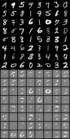
Image generated by Epoch1
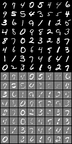
Image generated by Epoch10
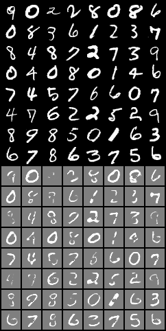
Image generated by Epoch30
The results show that the training is getting better slowly, but it is still a little vague. The effect of using VAE may be better.