Pytorch autoencoder (self coding, unsupervised learning)
1, Compression and decompression
There is a neural network. What it is doing is receiving a picture, then coding it, and finally restoring it from the coded picture
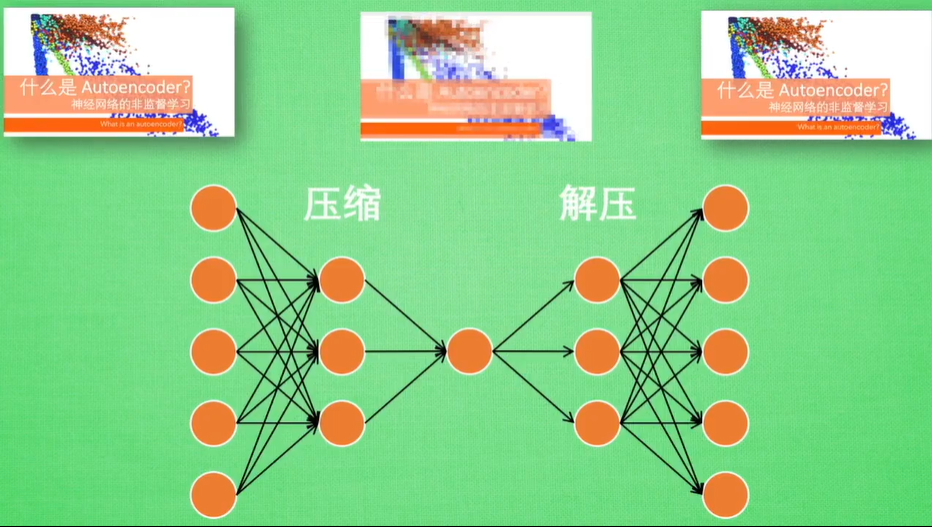
Assuming that the neural network is like this, corresponding to the picture just above, we can see that the picture is actually compressed and then decompressed When compressed, the original picture quality is reduced. When decompressed, the original picture is restored with a file with small amount of information but containing all key information Why?
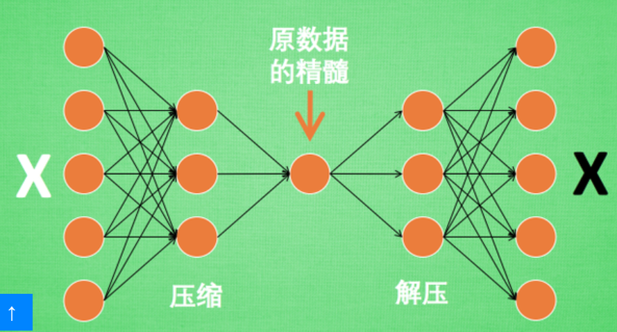
It turns out that sometimes the neural network needs to accept a large amount of input information. For example, when the input information is high-definition pictures, the amount of input information may reach tens of millions. It is a hard work for the neural network to learn directly from tens of millions of information sources So why not compress it, extract the most representative information in the original picture, reduce the amount of input information, and then put the reduced information into neural network for learning In this way, learning is simple and easy Therefore, self coding can play a role at this time The white X of the original data is compressed and decompressed into black x, and then the prediction error is calculated by comparing the black and white x, and the reverse transmission is carried out to gradually improve the accuracy of self coding The middle part of the trained self coding can summarize the essence of the original data It can be seen that from beginning to end, we only use the input data X and do not use the data label corresponding to X. therefore, it can also be said that self coding is an unsupervised learning It's time to really use self coding Usually only the first half of self coding is used
2, Encoder
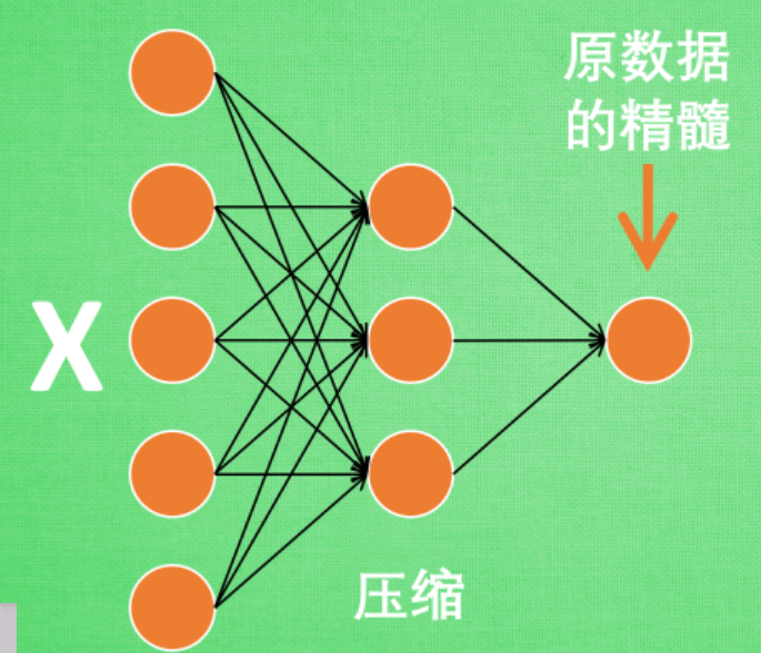
This part is also called encoder The encoder can get the essence of the original data, and then we only need to create a small neural network to learn the essence of the data, which not only reduces the burden of the neural network, but also achieves good results
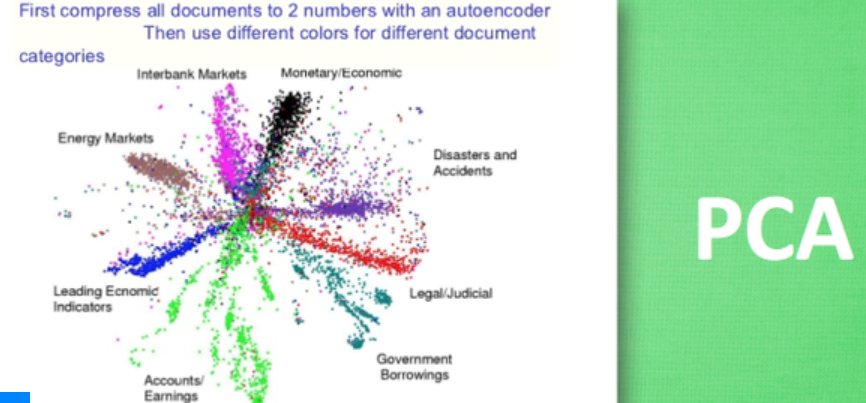
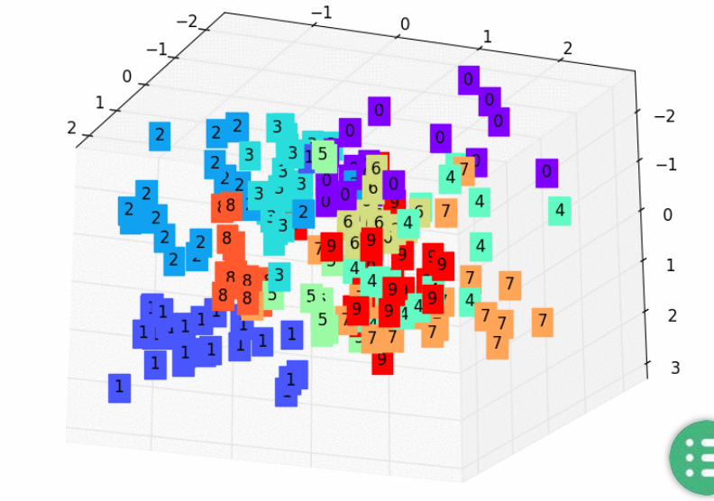
This is a data sorted out by self coding. It can summarize the characteristics of each type of data from the original data. If these feature types are placed on a two-dimensional picture, each type has been well distinguished by the essence of the original data If you understand PCA principal component analysis and then extract the main features, self coding is the same as it, even beyond PCA In other words, self coding can reduce the dimension of feature attributes like PCA
3, Decoder
As for the Decoder, we can also do something with it We know that the Decoder needs to decompress the essence information into the original information during training, so it provides the function of a decompressor. We can even think of it as a generator (similar to GAN )A special self coding for doing this is called variable autoencoders. You can here Find his specific instructions
An example is to make it imitate and generate handwritten numerals

4, Actual combat
main points
Neural network can also carry out unsupervised learning, only need training data, do not need label data Self coding is such a form Self coding can automatically classify data, and can also be nested on semi supervised learning, learning with a small number of labeled samples and a large number of unlabeled samples
This time we also use MNIST handwritten digital data to compress and decompress the pictures
Then the compressed features are used for unsupervised classification
1. Training data
For self coding, only the training set is needed, and only the image of training data needs to be trained instead of labels
2,AutoEncoder
The form of AutoEncoder is very simple. They are encoder and decoder respectively. They are compressed and decompressed. After compression, the compressed eigenvalues are obtained, and then the compressed eigenvalues are decompressed into the original picture
3. Training
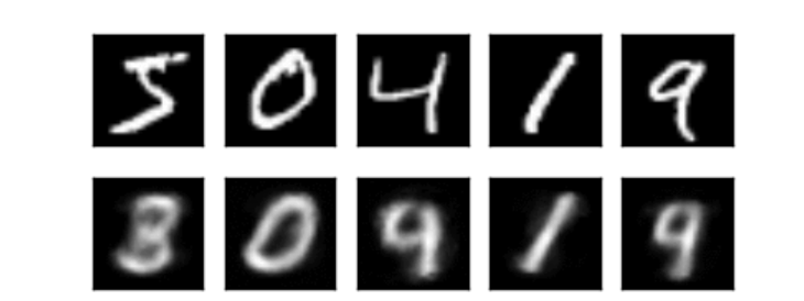
Training, and visualize the training process We can effectively use encoder and decoder to do many things. For example, here we use the information output of decoder to see the comparison with the original picture, and also use encoder to see the neural network's understanding of the original picture after compression Encoder can roughly separate different image data This is an unsupervised learning process
Full code:
import torch
import torch.nn as nn
import torch.utils.data as Data
import torchvision
import matplotlib.pyplot as plt
from mpl_toolkits.mplot3d import Axes3D
from matplotlib import cm
import numpy as np

# Super parameter
EPOCH = 10
BATCH_SIZE = 64
LR = 0.005
DOWNLOAD_MNIST = False   # If the data is downloaded, it can be set to False
N_TEST_IMG = 5          # At that time, 5 pictures will be displayed to see the effect, as shown in Figure 1 above

# Mnist digits dataset
train_data = torchvision.datasets.MNIST(
    root='./mnist/',
    train=True,                                     # this is training data
    transform=torchvision.transforms.ToTensor(),    # Converts a PIL.Image or numpy.ndarray to
                                                    # torch.FloatTensor of shape (C x H x W) and normalize in the range [0.0, 1.0]
    download=DOWNLOAD_MNIST,                        # download it if you don't have it
)

train_loader = Data.DataLoader(dataset=train_data, batch_size=BATCH_SIZE, shuffle=True)


# Self coding
class AutoEncoder(nn.Module):
    def __init__(self):
        super(AutoEncoder, self).__init__()

        # compress
        self.encoder = nn.Sequential(
            nn.Linear(28*28, 128),
            nn.Tanh(),  # activation
            nn.Linear(128, 64),
            nn.Tanh(),
            nn.Linear(64, 12),
            nn.Tanh(),
            nn.Linear(12, 3),   # Compressed into 3 features for 3D image visualization
        )
        # decompression
        self.decoder = nn.Sequential(
            nn.Linear(3, 12),
            nn.Tanh(),
            nn.Linear(12, 64),
            nn.Tanh(),
            nn.Linear(64, 128),
            nn.Tanh(),
            nn.Linear(128, 28*28),
            nn.Sigmoid(),       # The excitation function makes the output value in (0, 1)
        )

    def forward(self, x):
        encoded = self.encoder(x)
        decoded = self.decoder(encoded)
        return encoded, decoded


autoencoder = AutoEncoder()

optimizer = torch.optim.Adam(autoencoder.parameters(), lr=LR)
loss_func = nn.MSELoss()
# initialize figure
f, a = plt.subplots(2, N_TEST_IMG, figsize=(5, 2))
plt.ion()   # continuously plot

# original data (first row) for viewing
view_data = train_data.train_data[:N_TEST_IMG].view(-1, 28*28).type(torch.FloatTensor)/255.
for i in range(N_TEST_IMG):
    a[0][i].imshow(np.reshape(view_data.data.numpy()[i], (28, 28)), cmap='gray'); a[0][i].set_xticks(()); a[0][i].set_yticks(())

for epoch in range(EPOCH):
    for step, (x, b_label) in enumerate(train_loader):
        b_x = x.view(-1, 28*28)   # batch x, shape (batch, 28*28)
        b_y = x.view(-1, 28*28)   # batch y, shape (batch, 28*28)

        encoded, decoded = autoencoder(b_x)

        loss = loss_func(decoded, b_y)      # mean square error
        optimizer.zero_grad()               # clear gradients for this training step
        loss.backward()                     # backpropagation, compute gradients
        optimizer.step()                    # apply gradients

        if step % 100 == 0:
            print('Epoch: ', epoch, '| train loss: %.4f' % loss.data.numpy())

            # plotting decoded image (second row)
            _, decoded_data = autoencoder(view_data)
            for i in range(N_TEST_IMG):
                a[1][i].clear()
                a[1][i].imshow(np.reshape(decoded_data.data.numpy()[i], (28, 28)), cmap='gray')
                a[1][i].set_xticks(());
                a[1][i].set_yticks(())
            plt.draw();
            plt.pause(0.05)
plt.ioff()
plt.show()


# Data to view
view_data = train_data.train_data[:200].view(-1, 28*28).type(torch.FloatTensor)/255.
encoded_data, _ = autoencoder(view_data)    # Extract compressed eigenvalues
fig = plt.figure(2)
ax = Axes3D(fig)    # 3D diagram
# x. Data value of Y, Z
X = encoded_data.data[:, 0].numpy()
Y = encoded_data.data[:, 1].numpy()
Z = encoded_data.data[:, 2].numpy()
values = train_data.train_labels[:200].numpy()  # Tag value
for x, y, z, s in zip(X, Y, Z, values):
    c = cm.rainbow(int(255*s/9))    # Coloring
    ax.text(x, y, z, s, backgroundcolor=c)  # Marker
ax.set_xlim(X.min(), X.max())
ax.set_ylim(Y.min(), Y.max())
ax.set_zlim(Z.min(), Z.max())
plt.show()