[1] The function Gaussian mixture in machine learning solves the components of each model

[1.1] Gaussian texture parameter interpretation

Available references: [sklearn] detailed explanation of various parameters and code implementation of mixture. Gaussian mixture_ Yakuho blog - CSDN blog_ gaussianmixture

 

 

 

 

  [1.2] solution of single Gaussian model

from matplotlib import colors
import numpy as np
import matplotlib.pyplot as plt
from numpy.lib.twodim_base import diag
from sklearn.mixture import GaussianMixture

import numpy as np
import matplotlib.pyplot as plt

#mean value
def average(data):
    return np.sum(data)/len(data)
#standard deviation
def sigma(data,avg):
    sigma_squ=np.sum(np.power((data-avg),2))/len(data)
    return np.power(sigma_squ,0.5)
#Gaussian distribution probability
def prob(data,avg,sig):
    print(data)
    sqrt_2pi=np.power(2*np.pi,0.5)
    coef=1/(sqrt_2pi*sig)
    powercoef=-1/(2*np.power(sig,2))
    mypow=powercoef*(np.power((data-avg),2))
    return coef*(np.exp(mypow))
#sample data 
data=np.array([0.79,0.78,0.8,0.79,0.77,0.81,0.74,0.85,0.8
               ,0.77,0.81,0.85,0.85,0.83,0.83,0.8,0.83,0.71,0.76,0.8])
#Calculate the average of Gaussian distribution according to the sample data
ave=average(data)
#Calculate the standard deviation of Gaussian distribution according to the sample
sig=sigma(data,ave)
#Get the data
x=np.arange(0.5,1.0,0.01)
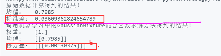
print("The result of original data calculation!")
print("Mean value:  ",ave)
print("Standard deviation:",sig)
# p=prob(x,ave,sig)
# plt.plot(x,p)
# plt.grid()
# plt.xlabel("apple quality factor")
# plt.ylabel("prob density")
# plt.yticks(np.arange(0,12,1))
# plt.title("Gaussian distrbution")
# plt.show()

#The results obtained by calling the Gaussian mixture function solution method in machine learning
'''
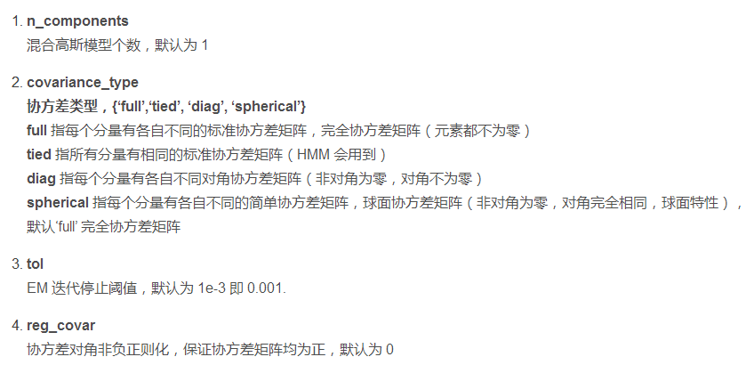
full It means that each component has its own different standard covariance matrix, complete covariance matrix (elements are not zero)
tied It means that all components have the same standard covariance matrix( HMM (will be used)
diag It means that each component has its own different diagonal covariance matrix (non diagonal zero, diagonal non-zero)
spherical It means that each component has its own different simple covariance matrix, spherical covariance matrix (non diagonal is zero, the diagonal is exactly the same, and the spherical characteristic), default'full' Complete covariance matrix
'''
gmm=GaussianMixture(n_components=1,covariance_type="diag",max_iter=100)
dataall=np.array(data,np.newaxis).reshape(-1,1)
gmm.fit(dataall)
print("Call in machine learning GaussianMixture The results obtained by the mixed function solution method!")
print("Weight:  ",gmm.weights_)
print("Mean value:  ",gmm.means_ )
print("Covariance:",gmm.covariances_)

Operation results

  Result analysis:

(1) It is found that the result of Gaussian mixture fitting is consistent with the result of original data calculation;

(2) According to the definition of covariance, the covariance of the variable to itself is the square of the standard deviation, so 0.0013 = 0.036 * 0.036

(3)   The results of Gaussian mixture cannot obtain the standard deviation of a single model, but only the covariance. The standard deviation of a single variable can be calculated by setting the type.

full means that each component has its own standard covariance matrix, complete covariance matrix (elements are not zero)

tied means that all components have the same standard covariance matrix (HMM will use it)

diag means that each component has its own different diagonal covariance matrix (non diagonal zero, diagonal non-zero)

Spherical means that each component has its own simple covariance matrix, spherical covariance matrix (non diagonal is zero, the diagonal is exactly the same, and the spherical characteristics)

[1.3] solution of hybrid GMM model

Generate three Gauss mixture models, and then call GaussianMixture to solve the weight, variance and covariance.

import numpy as np
import matplotlib.pyplot as plt
from gmm_em import gmm_em
from gmm_em import gaussian
from sklearn.neighbors import KernelDensity
from sklearn.mixture import GaussianMixture

D = 1 # 2d data
K = 3 # 3 mixtures

#1:
n1 = 70
mu1 = [0]
sigma2_1 = [[0.3]]
#2:
n2 = 150
mu2 = [2]
sigma2_2  = [[0.2]]
#3:
n3 = 100
mu3 = [4]
sigma2_3  = [[0.3]]

N = n1 + n2 + n3
alpha1 = n1/N
alpha2 = n2/N
alpha3 = n3/N


sample1 = np.random.multivariate_normal(mean=mu1, cov=sigma2_1, size=n1)
sample2 = np.random.multivariate_normal(mean=mu2, cov=sigma2_2, size=n2)
sample3 = np.random.multivariate_normal(mean=mu3, cov=sigma2_3, size=n3)


#Calculate the mean and variance of the original data
all_data=[sample1,sample2,sample3]
real_mean=[]
real_sigma=[]
for data in all_data:
    mean=np.sum(data)/len(data)
    real_mean.append(mean)
for index, data in enumerate(all_data) :
    sigma_squ=np.sum(np.power((data-real_mean[index]),2))/len(data)
    sigma=np.power(sigma_squ,0.5)
    real_sigma.append(sigma)
print("Mean value of original data:",real_mean)
print("Original data variance:",real_sigma)
Y = np.concatenate((sample1, sample2, sample3),axis=0)
Y_plot = np.linspace(-2, 6, 1000)[:, np.newaxis]
true_dens = (alpha1 * gaussian(Y_plot[:, 0], mu1, sigma2_1)
             + alpha2 * gaussian(Y_plot[:, 0], mu2, sigma2_2)
             + alpha2 * gaussian(Y_plot[:, 0], mu3, sigma2_3))

fig, ax = plt.subplots()
ax.fill(Y_plot[:, 0], true_dens, fc='black', alpha=0.2, label='true distribution')
ax.plot(sample1[:, 0], -0.005 - 0.01 * np.random.random(sample1.shape[0]), 'b+', label="input class1")
ax.plot(sample2[:, 0], -0.005 - 0.01 * np.random.random(sample2.shape[0]), 'r+', label="input class2")
ax.plot(sample3[:, 0], -0.005 - 0.01 * np.random.random(sample3.shape[0]), 'g+', label="input class3")

kernel = 'gaussian'
kde = KernelDensity(kernel=kernel, bandwidth=0.5).fit(Y)
log_dens = kde.score_samples(Y_plot)
ax.plot(Y_plot[:, 0], np.exp(log_dens), '-', label="input distribution".format(kernel))

ax.set_xlim(-2, 6)

# plt.show()

omega, alpha, mu, cov = gmm_em(Y, K, 100)

category = omega.argmax(axis=1).flatten().tolist()
class1 = np.array([Y[i] for i in range(N) if category[i] == 0])
class2 = np.array([Y[i] for i in range(N) if category[i] == 1])
class3 = np.array([Y[i] for i in range(N) if category[i] == 2])

est_dens = (alpha[0] * gaussian(Y_plot[:, 0], mu[0], cov[0])
             + alpha[1] * gaussian(Y_plot[:, 0], mu[1], cov[1])
             + alpha[2] * gaussian(Y_plot[:, 0], mu[2], cov[2]))

ax.fill(Y_plot[:, 0], est_dens, fc='blue', alpha=0.2, label='estimated distribution')
ax.plot(class1[:, 0], -0.03 - 0.01 * np.random.random(class1.shape[0]), 'bo', label="estimated class1")
ax.plot(class2[:, 0], -0.03 - 0.01 * np.random.random(class2.shape[0]), 'ro', label="estimated class2")
ax.plot(class3[:, 0], -0.03 - 0.01 * np.random.random(class3.shape[0]), 'go', label="estimated class3")
plt.legend(loc="best")
plt.title("GMM Data")
# plt.show()

#Errors:
# print("initialization weight:", alpha1, alpha2, alpha3)
# print("EM estimated weight:", alpha[0], alpha[1], alpha[2])

# print("initialization mean:", mu1, mu2, mu3)
# print("EM estimated mean:", mu[0], mu[1], mu[2])

# print("initialization covariance:", sigma2_1, sigma2_2, sigma2_3)
# print("EM estimated covariance:", cov[0], cov[1], cov[2])

gmm=GaussianMixture(n_components=3,covariance_type="diag",max_iter=100)
# dataall=np.array(Y,np.newaxis).reshape(-1,1)
gmm.fit(Y)
a=np.array(gmm.weights_)
b=np.array(gmm.means_)
c=np.array(gmm.covariances_)

print("Call in machine learning GaussianMixture The results obtained by the mixed function solution method!")
print("Weight:  ",a.reshape(1,-1))
print("Mean value:  ",b.reshape(1,-1))
print("Covariance:",c.reshape(1,-1))

Result printing

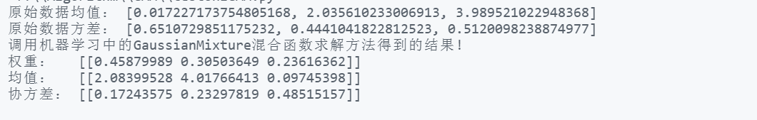
  Analysis: the mean and variance generated by Gaussian mixture are different from the mean and variance of the original data, because the mean variance solved by the hybrid model will be affected by other models, that is, from the perspective of integrity, it is different from the original distribution.

Question: how to calculate the standard deviation of a single model according to the calculated covariance?

Is the covariance of a single variable obtained in the mixed model the square of the standard deviation of a single model?? To be verified

[2] Iterative solution of Gaussian mixture model by EM algorithm

Derivation of Gaussian mixture model (GMM) and EM algorithm

code: