Summary of Wu Enda's Machine Learning Programming Jobs--Logistic Regression with Neural Network Thinking

The goal of machine learning is not to infuse knowledge into the machine, but to enable the machine to discover the rules by itself, even those that are difficult for human beings to discover.

1. Cat tutorial

1.1 Training Set and Test Set Introduction

train_set_x_orig: The image data in the training set (209 64x64 images in this training set) is saved.
train_set_y_orig: Save the corresponding classification value of the image of the training set ([0 | 1], 0 means not a cat, 1 means a cat).
Using np.squeeze to compress dimensions, only compressed values can be decoded
test_set_x_orig: Save the image data from the test set (this training set has 50 64x64 images).
test_set_y_orig: Save the corresponding classification values for the image of the test set ([0 | 1], 0 means not a cat, 1 means a cat).
classes: Save two string data of type bytes: [b'non-cat'b'cat'].
Width/height of each picture: num_px = 64
Size of each picture: (64, 64, 3)
Training Set_Dimension of Pictures: (209, 64, 64, 3)
Dimension of training set_label: (1, 209)
Test Set_Dimensions of Pictures: (50, 64, 64, 3)
Dimension of test set_label: (1, 50)

# Note: pycharm opens the training set picture
plt.figure("Image")
plt.imshow(train_set_x_orig[index])
plt.axis('on')
plt.title('image')
plt.show()

1.2 Picture data processing

1.2.1 Dimension reduction for pictures, transpose:

X_flatten = X.reshape(X.shape [0]，-1).T
# The last dimension of training set dimension reduction: (12288, 209)
# Dimensions after dimension reduction of test set: (12288, 50)

1.2.2 Standardized, dividing each row of picture data by 255 to place it between 0-1:

train_set_x = train_set_x_flatten / 255
test_set_x = test_set_x_flatten / 255

1.3 Sigmoid function

The Sigmoid function is often used as a threshold function of a neural network to map variables between 0 and 1
Shape: S-shaped
Function: s = 1/ (1 + np.exp(-z))

1.4 Propagation Function (Difficulty)

The main steps to build a neural network are:

1. Define the model structure (such as the number of input features)
2. Initialize model parameters
3. Cycle:
   3.1 Calculate current loss (forward propagation)
   3.2 Calculate the current gradient (reverse propagation)
   3.3 Update parameters (gradient descent)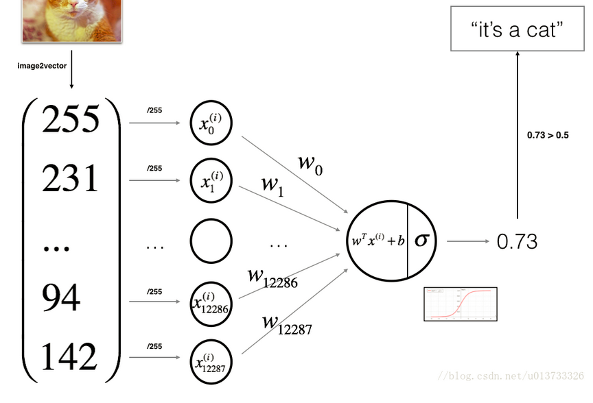
   
   Cost function and its gradient function propagate(), Note Update:

def propagate(w, b, X, Y):
	"""
	//Parameters:
	    w  - Weights, arrays of varying sizes (12288,1)
	    b  - Deviation, a scalar
	    X  - Picture Matrix, Matrix Type (12288, 209)
	    Y  - Tag matrix, true "tag" vector (non-cat 0, cat 1), matrix dimension is(1,209)
	
	//Return:
	    cost - Negative Logarithmic Cost of Logistic Regression
	    dw  - Be relative to w The loss gradient, therefore, corresponds to the w Same shape (12288, 1)
	    db  - Be relative to b The loss gradient, therefore, corresponds to the b Same shape
	"""
	
	# A two-dimensional array with y.shape[0] representing the number of rows and y.shape[1] representing the number of columns.
	m = X.shape[1] 
	
	# numpy syntax: dot: matrix multiplication, log: base e
	
	# Forward Propagation, z(i)=wT x(i)+b
	
	A = sigmoid(np.dot(w.T, X) + b)  
	# Calculate the activation value y^(i)=a(i)=sigmoid(z(i))
	
	cost = (- 1 / m) * np.sum(Y * np.log(A) + (1 - Y) * (np.log(1 - A)))
	# Calculate cost
	# Loss function L(a(i), y(i)=y(i) log(a(i)y(i)) log(1_y(i))log(1_a(i)) 
	# Cost J=1/m(i=1~m) L(a(i),y(i))
	
	# Reverse Propagation
	
	# da = dL(a,y)/da = -(y/a)+(1-y/1-a)
	# dz = dL(a,y)/dz = a-y
	# dw = 1/m X dzT    dw(i) = x(i)dz
	# db = 1/m ∑(i=1~m) dz(i)
	
	dw = (1 / m) * np.dot(X, (A - Y).T) 
	db = (1 / m) * np.sum(A - Y)
	
	# Use assertions to make sure my data is correct
    assert (dw.shape == w.shape)
    assert (db.dtype == float)
    cost = np.squeeze(cost)
    assert (cost.shape == ())

    # Create a dictionary and save dw and db.
    grads = {
        "dw": dw,
        "db": db
    }
    return grads, cost

1.5 optimize Function

Optimize w and b (weights and deviations) num_iterations (number of iterations) by the incoming learning_rate.Print cost every 100 times.It is divided into the following two steps and traversed:

1. Calculate the cost and gradient of the current parameter using propagate ().
2. Update the parameters using the gradient descent rule for w and b.

def optimize(w, b, X, Y, num_iterations, learning_rate, print_cost=False): 
    costs = []
    for i in range(num_iterations): 
    
        grads, cost = propagate(w, b, X, Y) 
        
        dw = grads["dw"]
        db = grads["db"]
        
        w = w - learning_rate * dw
        b = b - learning_rate * db 
        
        # Record costs every 100 times and print as needed
        if i % 100 == 0:
            costs.append(cost) 
            
        if print_cost and (i % 100 == 0):
            print("Number of iterations: %i ， Error value: %f" % (i, cost)) 
    params = {
        "w": w,
        "b": b}
    grads = {
        "dw": dw,
        "db": db}
    return (params, grads, costs)

1.6 Prediction function (predict):

Use the trained W and B to predict if the picture is a cat by sigmoid(w.T * X + b):?

def predict(w, b, X): 
    m = X.shape[1]  # Number of pictures
    Y_prediction = np.zeros((1, m))
    w = w.reshape(X.shape[0], 1)

    # Predict the probability of cats appearing in the picture
    A = sigmoid(np.dot(w.T, X) + b)

    for i in range(A.shape[1]):
        # Converting probability a [0, i] to actual prediction p [0, i]
        Y_prediction[0, i] = 1 if A[0, i] > 0.5 else 0
    return Y_prediction

1.7 model function:

Integrate previous functions, complete and beautiful (probably):

def model(X_train, Y_train, X_test, Y_test, num_iterations=2000, learning_rate=0.5, print_cost=False): 
#Initialization
    # This function creates a 0 vector with a dimension of (dim, 1) for w and initializes b to 0.
    w, b = initialize_with_zeros(X_train.shape[0])

#train
	# Optimize w and b
    parameters, grads, costs = optimize(w, b, X_train, Y_train, num_iterations, learning_rate, print_cost)

    # Get w and b
    w, b = parameters["w"], parameters["b"]

    # Forecast
    Y_prediction_test = predict(w, b, X_test)
    Y_prediction_train = predict(w, b, X_train)

    # Printing Accuracy
    print("Training set accuracy:", format(100 - np.mean(np.abs(Y_prediction_train - Y_train)) * 100), "%")
    print("Test Set Accuracy:", format(100 - np.mean(np.abs(Y_prediction_test - Y_test)) * 100), "%")

    d = {
        "costs": costs,
        "Y_prediction_test": Y_prediction_test,
        "Y_prediciton_train": Y_prediction_train,
        "w": w,
        "b": b,
        "learning_rate": learning_rate,
        "num_iterations": num_iterations}
    return d

1.8 Tests, drawings; Change learning rate and redraw:

print("====================test model====================")
# The actual data is loaded here, see the code section above.
d = model(train_set_x, train_set_y, test_set_x, test_set_y, num_iterations=2000, learning_rate=0.005, print_cost=True)

# Drawing
costs = np.squeeze(d['costs'])
plt.plot(costs)
plt.ylabel('cost')
plt.xlabel('iterations (per hundreds)')
plt.title("Learning rate =" + str(d["learning_rate"]))
plt.show()

learning_rates = [0.01, 0.001, 0.0001]
models = {}
for i in learning_rates:
    print("learning rate is: " + str(i))
    models[str(i)] = model(train_set_x, train_set_y, test_set_x, test_set_y,
                           num_iterations=1500, learning_rate=i, print_cost=False)
    print('\n' + "-------------------------------------------------------" + '\n')

for i in learning_rates:
    plt.plot(np.squeeze(models[str(i)]["costs"]), label=str(models[str(i)]["learning_rate"]))

plt.ylabel('cost')
plt.xlabel('iterations')

legend = plt.legend(loc='upper center', shadow=True)
frame = legend.get_frame()
frame.set_facecolor('0.90')
plt.show()