In the field of image processing, binary images are widely used because of their low computational complexity and their ability to represent the key features of images. The common method to change gray image into binary image is to select a threshold value, and then to process each pixel of the image to be processed by a single point, that is, to compare its gray value with the threshold set, so as to obtain a binary black-and-white image. Because of its intuitiveness and easy implementation, this method has been in the central position in the field of image segmentation. This paper summarizes the thresholding image segmentation algorithms that the author has learned in recent years, describes the author's understanding of each algorithm, and implements these algorithms based on OpenCV and VC 6.0. Finally, the source code will be open, I hope you can make progress together. (The code in this article does not consider execution efficiency for the time being)
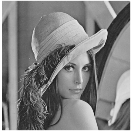
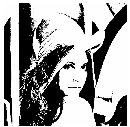
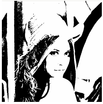
Firstly, the image to be segmented is given as follows:
1. Otsu Method (Maximum Interclass Variance Method)
This algorithm is a dynamic threshold segmentation algorithm proposed by Japanese Otsu. Its main idea is to divide the image into two parts: background and target according to the gray level characteristics, and to select the threshold value to maximize the variance between background and target. (The greater the variance between the background and the target, the greater the difference between the two parts. When part of the target is misclassified as background or part of the background is misclassified as target, the difference between the two parts will become smaller. Therefore, using the segmentation with the largest variance between classes means that the probability of misclassification is the smallest.) This is the main idea of this method. Its main realization principles are as follows:
1) Establishing gray histogram of image (there are L gray levels, each occurrence probability is p)
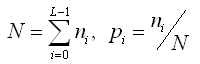
(2) Calculate the probability of background and target occurrence. The calculation method is as follows:
Suppose t is the selected threshold, A represents the background (gray level is 0~N). According to the elements in the histogram, Pa is the probability of background occurrence, B is the goal, and Pb is the probability of target occurrence.
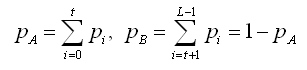
3) Calculate the inter-class variance between regions A and B as follows:
The first expression calculates the average gray values of A and B regions respectively.
The second expression calculates the global average gray level of the gray image.
The third expression calculates the inter-class variance between regions A and B.
4) The inter-class variance of a single gray value is calculated in the above steps, so the optimal threshold value should be the gray value that can maximize the inter-class gray variance of A and B in the image. In the program, it is necessary to optimize the gray value of each occurrence.
My VC implementation code is as follows.
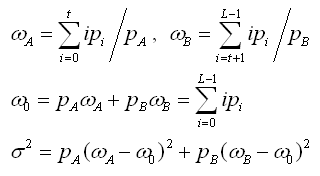
The result of threshold segmentation is shown in the following figure, and the threshold value is 116.
- /*****************************************************************************
- *
- * \Function name:
- * OneDimentionOtsu()
- *
- * \Input parameters:
- * pGrayMat: Binary image data
- * width: Graphic Dimension Width
- * height: Graphic Dimension Height
- * nTlreshold: Binary Segmentation Threshold after Algorithmic Processing
- * \Return value:
- * nothing
- * \Function Description: Realize the Binary Segmentation of Gray Gray Gray Gray Image - Maximum Interclass Variance Method (Otsu algorithm, commonly known as Otsu algorithm)
- *
- ****************************************************************************/
- void CBinarizationDlg::OneDimentionOtsu(CvMat *pGrayMat, int width, int height, BYTE &nThreshold)
- {
- double nHistogram[256]; //Gray histogram
- double dVariance[256]; //Interclass variance
- int N = height*width; //Total Pixel Number
- for(int i=0; i<256; i++)
- {
- nHistogram[i] = 0.0;
- dVariance[i] = 0.0;
- }
- for(i=0; i<height; i++)
- {
- for(int j=0; j<width; j++)
- {
- unsigned char nData = (unsigned char)cvmGet(pGrayMat, i, j);
- nHistogram[nData]++; //Establishing Histogram
- }
- }
- double Pa=0.0; //Background occurrence probability
- double Pb=0.0; //Target occurrence probability
- double Wa=0.0; //Background average gray value
- double Wb=0.0; //Target average gray value
- double W0=0.0; //Global average gray value
- double dData1=0.0, dData2=0.0;
- for(i=0; i<256; i++) //Computing Global Average Gray Level
- {
- nHistogram[i] /= N;
- W0 += i*nHistogram[i];
- }
- for(i=0; i<256; i++) //Calculate the variance between classes for each gray value
- {
- Pa += nHistogram[i];
- Pb = 1-Pa;
- dData1 += i*nHistogram[i];
- dData2 = W0-dData1;
- Wa = dData1/Pa;
- Wb = dData2/Pb;
- dVariance[i] = (Pa*Pb* pow((Wb-Wa), 2));
- }
- //Traverse each variance to get the gray value corresponding to the maximum variance between classes
- double temp=0.0;
- for(i=0; i<256; i++)
- {
- if(dVariance[i]>temp)
- {
- temp = dVariance[i];
- nThreshold = i;
- }
- }
- }
2. One-dimensional cross-entropy method
Similar to the maximum variance between classes, this method was developed by Li and Lee applying the theory of entropy in information theory. Firstly, the concept of cross-entropy is briefly introduced.
For two distributions P and Q, the information cross-entropy D is defined as follows: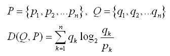
The physical meaning of this representation is the theoretical distance of information between two distributions. Another understanding is the change of information brought about by changing the distribution P to Q. For image segmentation, if the original image is to be replaced by the segmented image, the optimal segmentation basis should be to minimize the cross-entropy between the two images. The following is a brief summary of the process of minimum cross-entropy method.
It can be assumed that P is the gray distribution of the source image and Q is the gray distribution of the segmented image.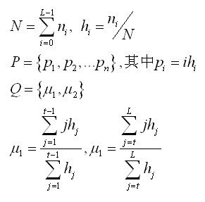
H is the statistical histogram in the formula above.
N is the total number of pixels in the image.
L is the total gray level of the source image.
P represents the source image, and each element represents the gray distribution (average gray value) at each gray level.
Q is the segmented binary image, and two u represent the average gray value of the two segmented regions respectively, where t is the threshold used for the segmented image.
According to the above definition, it is easy to deduce the quantitative expression of cross-entropy between P and Q based on the formula of cross-entropy with the sum of gray levels as the calculation amount.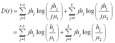
According to the idea mentioned above, the minimum t of D is the optimal threshold in the sense of minimum cross-entropy.
The author's VC implementation code is as follows.
- /*****************************************************************************
- *
- * \Function name:
- * MiniCross()
- *
- * \Input parameters:
- * pGrayMat: Binary image data
- * width: Graphic Dimension Width
- * height: Graphic Dimension Height
- * nTlreshold: Binary Segmentation Threshold after Algorithmic Processing
- * \Return value:
- * nothing
- * \Function Description: Realizing Binary Segmentation of Gray Gray Image-Minimum Cross Entropy Method
- *
- ****************************************************************************/
- void CBinarizationDlg::MiniCross(CvMat *pGrayMat, int width, int height, BYTE &nThreshold)
- {
- double dHistogram[256]; //Gray histogram
- double dEntropy[256]; //Cross Entropy of Each Pixel
- int N = height*width; //Total Pixel Number
- for(int i=0; i<256; i++)
- {
- dHistogram[i] = 0.0;
- dEntropy[i] = 0.0;
- }
- for(i=0; i<height; i++)
- {
- for(int j=0; j<width; j++)
- {
- unsigned char nData = (unsigned char)cvmGet(pGrayMat, i, j);
- dHistogram[nData]++; //Establishing Histogram
- }
- }
- double Pa=0.0; //Area 1 Average Gray Value
- double Pb=0.0; //Area 2 Average Gray Value
- double P0=0.0; //Global average gray value
- double Wa=0.0; //Part I Entropy
- double Wb=0.0; //Entropy of Part Two
- double dData1=0.0, dData2=0.0; //Intermediate value
- double dData3=0.0, dData4=0.0; //Intermediate value
- for(i=0; i<256; i++) //Computing Global Average Gray Level
- {
- dHistogram[i] /= N;
- P0 += i*dHistogram[i];
- }
- for(i=0; i<256; i++)
- {
- Wa=Wb=dData1=dData2=dData3=dData4=Pa=Pb=0.0;
- for(int j=0; j<256; j++)
- {
- if(j<=i)
- {
- dData1 += dHistogram[j];
- dData2 += j*dHistogram[j];
- }
- else
- {
- dData3 += dHistogram[j];
- dData4 += j*dHistogram[j];
- }
- }
- Pa = dData2/dData1;
- Pb = dData4/dData3;
- for(j=0; j<256; j++)
- {
- if(j<=i)
- {
- if((Pa!=0)&&(dHistogram[j]!=0))
- {
- double d1 = log(dHistogram[j]/Pa);
- Wa += j*dHistogram[j]*d1/log(2);
- }
- }
- else
- {
- if((Pb!=0)&&(dHistogram[j]!=0))
- {
- double d2 = log(dHistogram[j]/Pb);
- Wb += j*dHistogram[j]*d2/log(2);
- }
- }
- }
- dEntropy[i] = Wa+Wb;
- }
- //Ergodic Entropy Value and Gray Value of Minimum Cross Entropy
- double temp=dEntropy[0];
- for(i=1; i<256; i++)
- {
- if(dEntropy[i]<temp)
- {
- temp = dEntropy[i];
- nThreshold = i;
- }
- }
- }
The result of threshold segmentation is as follows: the threshold value obtained by solving the problem is 106.
3. Two-dimensional OTSU method
This method is an extension of the method of maximum variance between classes, which extends the maximum variance between two one-dimensional distributions to the maximum value of the trace of the matrix of interspecific dispersion, and adds the average pixel value of the neighborhood of the pixel point on the basis of considering the gray level of the pixel point.
Following is an analysis of the method's thinking and the pushing-down process according to my understanding:
1) First of all, we need to establish two-dimensional gray statistical histogram P(f, g);
If the gray level of the image is L-level, then the gray level of the average gray level of 8 neighborhoods of each pixel is L-level, and the histogram P is constructed accordingly. The horizontal axis of the two-dimensional statistical histogram is the gray value f(i, j) of each pixel, and the vertical coordinate is the average neighborhood value g(i, j) corresponding to the same point, where (0 < I < height, 0 < J < width, 0 < f(i, j) < L), while the gray value f of the corresponding P(f,g) image is the whole gray value of f, and the statistical value of the neighborhood gray mean value G is the proportion of the total pixels (i.e., the ratio of the neighborhood gray value of g). It is the joint probability density of gray value. Each element of P satisfies the following formula: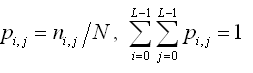
n is the statistic value of the gray value f in the whole image and the gray mean value g in the neighborhood.
N is the total number of pixels in the image.
2) For the two-dimensional statistical histogram shown in the following figure, t represents abscissa (gray value) and s represents ordinate (gray mean value of neighborhood of pixels)
For the threshold point (t,s) in an image, the difference between the gray value T and the gray mean s in its neighborhood should not be too large. If t is much larger than s (the point is located in the area II of the image above), it means that the gray value of the pixel is much larger than the gray mean of its neighborhood, so the point is likely to be a noise point, otherwise, if t is larger than S. It is much smaller (the point is located in the IV area on the way), that is, the pixel value of the point is much smaller than its neighborhood mean value, which means that it is an edge point. Therefore, we neglect these interference factors in background foreground segmentation, and consider that Pi,j=0 in these two regions. The remaining I and III regions represent the foreground and background respectively. Based on this, the optimal derivation of the discreteness criterion for the selected threshold (t,s) is derived.
3) Derivation of Discreteness Matrix Criteria at Threshold (t, s) Points
According to the analysis above, the probability of the occurrence of foreground and background segmented by threshold (t, s) is as follows:
Define two intermediate variables to facilitate the following derivation:

Accordingly, the gray mean vectors of these two parts can be deduced as follows (the two components are calculated according to the gray value and the gray mean of each point, respectively):

The gray mean vector of the whole image is:

In the same way as the one-dimensional Otsu method, we derive the variance between classes, which is two-dimensional, so we need to use the matrix form. Referring to the one-dimensional method, the "variance" matrix between classes can also be defined as follows:

In order to easily determine the "maximum" of such a matrix when it is implemented, the trace of the matrix (the sum of diagonals) is used to measure the "size" of the matrix in mathematics. Therefore, the trace of the matrix is used as the discreteness measure, and the derivation is as follows:

In this way, the optimal threshold combination can be obtained when the parameter is maximized (t,s).
The following is the implementation process of the algorithm:
1) Establishment of two-dimensional histogram
2) The histogram is traversed to calculate the matrix dispersion of each (t,s) combination, which is the so-called maximum inter-class variance in the one-dimensional Otsu method.
3) To get the maximum variance between classes (t,s). Since T represents the gray value and s represents the gray mean of the change point in its neighborhood, I think that s is the best choice when choosing the threshold, of course, t is also the best choice, because it can be seen from the solution results that this value is often very close.
The specific implementation code is as follows:
- /*****************************************************************************
- *
- * \Function name:
- * TwoDimentionOtsu()
- *
- * \Input parameters:
- * pGrayMat: Binary image data
- * width: Graphic Dimension Width
- * height: Graphic Dimension Height
- * nTlreshold: Binary Segmentation Threshold after Algorithmic Processing
- * \Return value:
- * nothing
- * \Function Description: Realizing Binary Segmentation of Gray Gray Gray Image - Maximum Interclass Variance Method (Two-Dimensional Otsu Algorithms)
- * \Note: When constructing two-dimensional histogram, the 3*3 neighborhood mean of gray points is used.
- ******************************************************************************/
- void CBinarizationDlg::TwoDimentionOtsu(CvMat *pGrayMat, int width, int height, BYTE &nThreshold)
- {
- double dHistogram[256][256]; //Establishment of two-dimensional gray histogram
- double dTrMatrix = 0.0; //Traces of Discrete Matrix
- int N = height*width; //Total Pixel Number
- for(int i=0; i<256; i++)
- {
- for(int j=0; j<256; j++)
- dHistogram[i][j] = 0.0; //initialize variable
- }
- for(i=0; i<height; i++)
- {
- for(int j=0; j<width; j++)
- {
- unsigned char nData1 = (unsigned char)cvmGet(pGrayMat, i, j); //Current gray value
- unsigned char nData2 = 0;
- int nData3 = 0; //Note that the sum of nine values may exceed one byte
- for(int m=i-1; m<=i+1; m++)
- {
- for(int n=j-1; n<=j+1; n++)
- {
- if((m>=0)&&(m<height)&&(n>=0)&&(n<width))
- nData3 += (unsigned char)cvmGet(pGrayMat, m, n); //Current gray value
- }
- }
- nData2 = (unsigned char)(nData3/9); //Zero-filling and Neighborhood Means for Overbound Index Values
- dHistogram[nData1][nData2]++;
- }
- }
- for(i=0; i<256; i++)
- for(int j=0; j<256; j++)
- dHistogram[i][j] /= N; //Get the normalized probability distribution
- double Pai = 0.0; //Mean Vector i Component in Target Area
- double Paj = 0.0; //j component of mean vector in target area
- double Pbi = 0.0; //Mean Vector i Component in Background Area
- double Pbj = 0.0; //Background mean vector j component
- double Pti = 0.0; //Global mean vector i component
- double Ptj = 0.0; //Global mean vector j component
- double W0 = 0.0; //Joint probability density of target area
- double W1 = 0.0; //Joint probability density of background region
- double dData1 = 0.0;
- double dData2 = 0.0;
- double dData3 = 0.0;
- double dData4 = 0.0; //Intermediate variable
- int nThreshold_s = 0;
- int nThreshold_t = 0;
- double temp = 0.0; //Seeking the Maximum
- for(i=0; i<256; i++)
- {
- for(int j=0; j<256; j++)
- {
- Pti += i*dHistogram[i][j];
- Ptj += j*dHistogram[i][j];
- }
- }
- for(i=0; i<256; i++)
- {
- for(int j=0; j<256; j++)
- {
- W0 += dHistogram[i][j];
- dData1 += i*dHistogram[i][j];
- dData2 += j*dHistogram[i][j];
- W1 = 1-W0;
- dData3 = Pti-dData1;
- dData4 = Ptj-dData2;
- /* W1=dData3=dData4=0.0; //Initialization of internal loop data
- for(int s=i+1; s<256; s++)
- {
- for(int t=j+1; t<256; t++)
- {
- W1 += dHistogram[s][t];
- dData3 += s*dHistogram[s][t]; //Method 2
- dData4 += t*dHistogram[s][t]; //You can also add loops to your calculations.
- }
- }*/
- Pai = dData1/W0;
- Paj = dData2/W0;
- Pbi = dData3/W1;
- Pbj = dData4/W1; //Two mean vectors are obtained and expressed by four components.
- dTrMatrix = ((W0*Pti-dData1)*(W0*Pti-dData1)+(W0*Ptj-dData1)*(W0*Ptj-dData2))/(W0*W1);
- if(dTrMatrix > temp)
- {
- temp = dTrMatrix;
- nThreshold_s = i;
- nThreshold_t = j;
- }
- }
- }
- nThreshold = nThreshold_t; //Returns the gray value in the result
- //nThreshold = 100;
- }
The result of threshold segmentation is as follows: the threshold obtained by solving is 114. (s=114, t=117)

References
[1] Nobuyuki Otsu. A Threshold SelectionMethod from Gray-Level Histograms.
[2] C. H. Li and C. K. Lee. Minimum CrossEntropy Thresholding
[3] Jian Gong, LiYuan Liand WeiNan Chen. Fast Recursive Algorithms For Two-Dimensional Thresholding.
Because the speed of the network is not enough, this article's formula and picture upload is slow. It's not easy to use the author for a long time. Therefore, if you want to reprint, please indicate the address of reprinting, in order to calculate the hard work of the author. At the same time, I hope to leave more messages and give the author points.
Reprinted at: https://www.cnblogs.com/hustkks/archive/2012/04/13/2445708.html