Record the details of a kaggle-based game, time series segmentation, feature construction, missing value processing.
Preface
This time, I participated in a credit card fraud prediction project on kaggle. I hope some details of the competition can be recorded and shared in order to avoid long forgetting.
Competition Address: https://www.kaggle.com/c/ieee-fraud-detection
data processing
Briefly describe the data characteristics of this competition:
1. 400 anonymous features
2. Some features have large-scale missing values.
3. Distribution of missing values in training and prediction data is quite different.
4. Characteristics of suspected time increment (to confirm)
5. Two kinds of anonymous data are given, one is about the card account information, the other is the card transaction information.
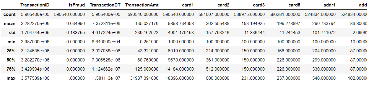
// An highlighted block
#Read data
train_id=pd.read_csv('data1/train_identity.csv')
test_id=pd.read_csv('data1/test_identity.csv')
train_data=pd.read_csv('data1/train_transaction.csv')
test_data=pd.read_csv('data1/test_transaction.csv')
#Combine the two types of data and clear the memory at the same time
train = train_data.merge(train_id, how='left', on='TransactionID')
test = test_data.merge(test_id, how='left',on='TransactionID')
del train_id; gc.collect()
del test_id; gc.collect()
del train_data; gc.collect()
del test_data; gc.collect()
train.describe()
train.isnull().sum()
TransactionID          0
isFraud                0
TransactionDT          0
TransactionAmt         0
ProductCD              0
card1                  0
card2               8933
card3               1565
card4               1577
card5               4259
card6               1571
addr1              65706
addr2              65706
dist1             352271
dist2             552913
P_emaildomain      94456
R_emaildomain     453249
C1                     0
C2                     0
C3                     0
C4                     0
C5                     0
C6                     0
C7                     0
C8                     0
C9                     0
C10                    0
C11                    0
C12                    0
C13                    0
                   ...
id_11             449562
id_12             446307
id_13             463220
id_14             510496
id_15             449555
id_16             461200
id_17             451171
id_18             545427
id_19             451222
id_20             451279
id_21             585381
id_22             585371
id_23             585371
id_24             585793
id_25             585408
id_26             585377
id_27             585371
id_28             449562
id_29             449562
id_30             512975
id_31             450258
id_32             512954
id_33             517251
id_34             512735
id_35             449555
id_36             449555
id_37             449555
id_38             449555
DeviceType        449730
DeviceInfo        471874
Length: 434, dtype: int64
Comparison of missing values between train and test:
training_missing = train.isna().sum(axis=0) / train.shape[0]
test_missing = test.isna().sum(axis=0) / test.shape[0]
change = (training_missing / test_missing).sort_values(ascending=False)
change = change[change<1e6] # remove the divide by zero errors
train_more=change[change>4].reset_index()
train_more.columns=['train_more_id','rate']
test_more=change[change<0.4].reset_index()
test_more.columns=['test_more_id','rate']
train_more_id=train_more['train_more_id'].values
train[train_more_id].head()
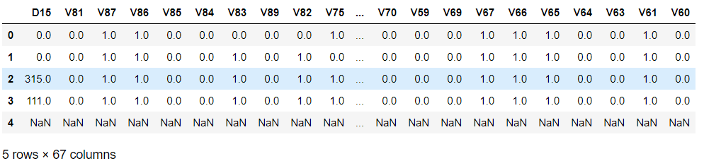
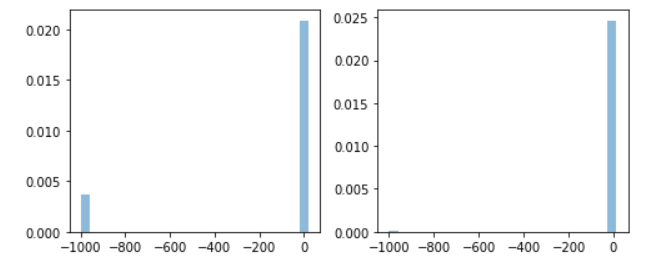
In comparison with V80, the missing values are filled in with -999. It is obvious that the number of train s missing after ["Transaction DT"]>2.5e7 is much higher than that of Test.
fig, axs = plt.subplots(ncols=2)

train_vals = train["V80"].fillna(-999)
test_vals = test[test["TransactionDT"]>2.5e7]["V80"].fillna(-999) # values following the shift


axs[0].hist(train_vals, alpha=0.5, normed=True, bins=25)

axs[1].hist(test_vals, alpha=0.5, normed=True, bins=25)


fig.set_size_inches(7,3)
plt.tight_layout()
Next, we make a simple analysis of the data.
-
Firstly, it can be observed in the data that most of the fraudulent users use'P_email domain'. Consider listing as a feature separately, and classify all kinds of mailboxes at the same time.
-
As mentioned earlier, Transaction DT is suspected of time increment. The maximum and minimum values of training and prediction set are subtracted, and 364 is obtained by removing'606024', while the training set is 182 and the prediction set is 182.
-
Obviously, the whole data is clean sequential cutting, that is, there is no duplicate time, so if we use datetime to deal with Transaction DT, only hour and weekend can help model training, other features such as MONTH in training may help you get good scores. However, the lack of prediction affects the accuracy of the model. ;
-
In this case, TimeSeries Split segmentation training and testing are used in the training model, which should be the key point of the game.
-
As mentioned earlier, the training and prediction sets are unevenly distributed when Transaction DT is greater than or equal to 2.5e7, which is also the key to get a good ranking.
-
The distribution of hour and isFraud is observed, showing a feature that is significantly higher from 1 to 6 points than other time points, and constructing'night'feature (considering the data based on one year, it is not helpful for feature extraction of seasons and holidays);
-
At the same time, for a user, the number of features missing is also related to the impact of isFraud (the more anonymous, the safer?). Add'isna'feature;
-
Data distribution and its imbalance have been attempted under-sampling and re-sampling as well as smote re-sampling, and the effect is relatively general. Especially under-sampling is lower than I expected, but the last choice is 1:5 under-sampling (after all, fast running, haha) plus classification penalty weight. The reason for adding weight is to classify more 0 into 1 after under-sampling.
Codeisna = train.isna().sum(axis=1)
isna_test = test.isna().sum(axis=1)
train['isna']=train.isna().sum(axis=1)
test['isna']=test.isna().sum(axis=1)import datetime START_DATE = '2017-12-01' startdate = datetime.datetime.strptime(START_DATE, '%Y-%m-%d') train['TransactionDT'] = train['TransactionDT'].apply(lambda x: (startdate + datetime.timedelta(seconds = x))) test['TransactionDT'] = test['TransactionDT'].apply(lambda x: (startdate + datetime.timedelta(seconds = x))) train['hour'] = train['TransactionDT'].dt.hour test['hour'] = test['TransactionDT'].dt.hour train['month'] = train['TransactionDT'].dt.month test['month'] = test['TransactionDT'].dt.month #print(train['TransactionDT']) x=test['hour']<7 x1=test['hour']>19 x.astype(int) x1.astype(int) x2=np.add(x,x1) x2.astype(int) test['night']=x2.astype(int) x=train['hour']<7 x1=train['hour']>19 x.astype(int) x1.astype(int) x2=np.add(x,x1) x2.astype(int) train['night']=x2.astype(int) index _pro=train['P_emaildomain']=='protonmail.com' index_pro_data=train['P_emaildomain'][index_pro] train['isprotonmail']=index_pro_data del index_pro del index_pro_data index_pro=test['P_emaildomain']=='protonmail.com' index_pro_data=test['P_emaildomain'][index_pro] test['isprotonmail']=index_pro_data del index_pro del index_pro_data train.loc[ (train.isprotonmail.isnull()), 'isprotonmail' ] = 0 train['isprotonmail'].describe(include="all") test.loc[ (test.isprotonmail.isnull()), 'isprotonmail' ] = 0 test['isprotonmail'].describe(include="all") emails = {'gmail': 'google', 'att.net': 'att', 'twc.com': 'spectrum', 'scranton.edu': 'other', 'optonline.net': 'other', 'hotmail.co.uk': 'microsoft', 'comcast.net': 'other', 'yahoo.com.mx': 'yahoo', 'yahoo.fr': 'yahoo', 'yahoo.es': 'yahoo', 'charter.net': 'spectrum', 'live.com': 'microsoft', 'aim.com': 'aol', 'hotmail.de': 'microsoft', 'centurylink.net': 'centurylink', 'gmail.com': 'google', 'me.com': 'apple', 'earthlink.net': 'other', 'gmx.de': 'other', 'web.de': 'other', 'cfl.rr.com': 'other', 'hotmail.com': 'microsoft', 'protonmail.com': 'other', 'hotmail.fr': 'microsoft', 'windstream.net': 'other', 'outlook.es': 'microsoft', 'yahoo.co.jp': 'yahoo', 'yahoo.de': 'yahoo', 'servicios-ta.com': 'other', 'netzero.net': 'other', 'suddenlink.net': 'other', 'roadrunner.com': 'other', 'sc.rr.com': 'other', 'live.fr': 'microsoft', 'verizon.net': 'yahoo', 'msn.com': 'microsoft', 'q.com': 'centurylink', 'prodigy.net.mx': 'att', 'frontier.com': 'yahoo', 'anonymous.com': 'other', 'rocketmail.com': 'yahoo', 'sbcglobal.net': 'att', 'frontiernet.net': 'yahoo', 'ymail.com': 'yahoo', 'outlook.com': 'microsoft', 'mail.com': 'other', 'bellsouth.net': 'other', 'embarqmail.com': 'centurylink', 'cableone.net': 'other', 'hotmail.es': 'microsoft', 'mac.com': 'apple', 'yahoo.co.uk': 'yahoo', 'netzero.com': 'other', 'yahoo.com': 'yahoo', 'live.com.mx': 'microsoft', 'ptd.net': 'other', 'cox.net': 'other', 'aol.com': 'aol', 'juno.com': 'other', 'icloud.com': 'apple'} us_emails = ['gmail', 'net', 'edu'] for c in ['P_emaildomain', 'R_emaildomain']: train[c + '_bin'] = train[c].map(emails) test[c + '_bin'] = test[c].map(emails) train[c + '_suffix'] = train[c].map(lambda x: str(x).split('.')[-1]) test[c + '_suffix'] = test[c].map(lambda x: str(x).split('.')[-1]) train[c + '_suffix'] = train[c + '_suffix'].map(lambda x: x if str(x) not in us_emails else 'us') test[c + '_suffix'] = test[c + '_suffix'].map(lambda x: x if str(x) not in us_emails else 'us') from sklearn.preprocessing import Imputer imp = Imputer(missing_values='NaN', strategy='most_frequent', axis=0)
Treatment of missing values
test[['dist1','dist2','C1','C2','C4','C5','C6','C7','C8','C9','C10','C11','C12','C13','C14']]=imp.fit_transform(test[['dist1','dist2','C1','C2','C4','C5','C6','C7','C8','C9','C10','C11','C12','C13','C14']])
train[['dist1','dist2','C1','C2','C4','C5','C6','C7','C8','C9','C10','C11','C12','C13','C14']]=imp.fit_transform(train[['dist1','dist2','C1','C2','C4','C5','C6','C7','C8','C9','C10','C11','C12','C13','C14']])
 test[test.TransactionDT>2.5e7][train_more_id]=imp.fit_transform(test[test.TransactionDT>2.5e7][train_more_id])
 train[train_more_id]=imp.fit_transform(train[train_more_id])
This part deals with a few missing data, and then some missing but important features are filled with random forest method. Here is only a piece of code.
from sklearn.ensemble import RandomForestRegressor
def set_missing_card2(df):
    # Remove existing numerical features and throw them into Random Forest Regressor
    give_df = df[['card2', 'TransactionID', 'card1', 'TransactionAmt', 'C1', 'C2',  'C4', 'C5', 'C6', 'C7', 'C8', 'C9', 'C10', 'C11', 'C12', 'C13']]
        # Passengers are divided into known age and unknown age.
        # ,'card3','card5','addr1''addr2'
    known_card2 = give_df[give_df.card2.notnull()].as_matrix()
    unknown_card2 = give_df[give_df.card2.isnull()].as_matrix()
        # y is the target age
    y = known_card2[:, 0]
    # X is the characteristic attribute value
    X = known_card2[:, 1:]
        # fit into Random Forest Regressor
    rfr = RandomForestRegressor(random_state=0, n_estimators=10, n_jobs=-1)
    rfr.fit(X, y)
        # Prediction of unknown age results using the obtained model
    predictedcard2= rfr.predict(unknown_card2[:, 1::])# One or two colons are the same.
        # Filling in the missing data with the predicted results
    df.loc[(df.card2.isnull()), 'card2']= predictedcard2
    return df, rfr
    # train_data.head()
train, rfr = set_missing_card2(train)
test, rfr = set_missing_card2(test)
Next, other missing feature values and dictionary character feature codes are processed.
for c1, c2 in train.dtypes.reset_index().values:
    if c2=='O':
        train[c1] = train[c1].map(lambda x: labels[str(x).lower()])
        test[c1] = test[c1].map(lambda x: labels[str(x).lower()])
train.fillna(-999, inplace=True)
test.fillna(-999, inplace=True)

for f in test.columns:                  #There are items in the train that need to be predicted, so I don't want to remove them and use test directly.
    if train[f].dtype=='object' or test[f].dtype=='object':
        print(f)
        lbl = preprocessing.LabelEncoder()
        lbl.fit(list(train[f].values) + list(test[f].values))
        train[f] = lbl.transform(list(train[f].values))
        test[f] = lbl.transform(list(test[f].values))
The original idea here was to separate the data by month and then do under/resampling. It was done by training for 4 months and testing for 2 months. Later, it was more convenient to directly divide the data into TimeSeries Split.
columns_list=list(train)
####Separating data sets by month
train_12=train[train.month==12]
train_1=train[train.month==1]
train_2=train[train.month==2]
train_3=train[train.month==3]
train_4=train[train.month==4]
train_5=train[train.month==5]
train_6=train[train.month==6]

from imblearn.under_sampling import RandomUnderSampler
ran=RandomUnderSampler(return_indices=True) ##intialize to return indices of dropped rows
train_12,y_train12,dropped12 = ran.fit_sample(train_12,train_12['isFraud'])
train_1,y_train1,dropped1 = ran.fit_sample(train_1,train_1['isFraud'])
train_2,y_train2,dropped2 = ran.fit_sample(train_2,train_2['isFraud'])
train_3,y_train3,dropped3 = ran.fit_sample(train_3,train_3['isFraud'])
train_4,y_train4,dropped4 = ran.fit_sample(train_4,train_4['isFraud'])
train_5,y_train5,dropped5 = ran.fit_sample(train_5,train_5['isFraud'])
train_6,y_train6,dropped6 = ran.fit_sample(train_6,train_6['isFraud'])
del train
del y_train12
del y_train1
del y_train2
del y_train3
del y_train4
del y_train5
del y_train6

'''#Random oversampling
from imblearn.over_sampling import RandomOverSampler
ros = RandomOverSampler(random_state=0)
train_data, y_train = ros.fit_sample(train, y_train)
del train; gc.collect()'''
'''#smote oversampling
from imblearn.over_sampling import SMOTE
smote = SMOTE(frac=0.1, random_state=1)
train_data, y_train = smote.fit_sample(train, y_train)'''

'''from imblearn.under_sampling import RandomUnderSampler
ran=RandomUnderSampler(return_indices=True) ##intialize to return indices of dropped rows
train_data,y_train,dropped = ran.fit_sample(train,y_train)
del train; gc.collect()'''
Model Construction Training Section
This time, we did not use SVM to play the game. We used the artifact XGBOOST. In two days, we will push XGBOOST by hand and post some adjustments. Here we will not go into details. Direct to the code on the document:
def fast_auc(y_true, y_prob):

    y_true = np.asarray(y_true)
    y_true = y_true[np.argsort(y_prob)]
    nfalse = 0
    auc = 0
    n = len(y_true)
    for i in range(n):
        y_i = y_true[i]
        nfalse += (1 - y_i)
        auc += y_i * nfalse
    auc /= (nfalse * (n - nfalse))
    return auc


def eval_auc(y_true, y_pred):

    return 'auc', fast_auc(y_true, y_pred), True


def group_mean_log_mae(y_true, y_pred, types, floor=1e-9):

    maes = (y_true-y_pred).abs().groupby(types).mean()
    return np.log(maes.map(lambda x: max(x, floor))).mean()
def train_model_classification(X, X_test, y, params, folds, model_type='lgb', eval_metric='auc', columns=None, plot_feature_importance=False, model=None,
                               verbose=10000, early_stopping_rounds=200, n_estimators=50000, splits=None, n_folds=3, averaging='usual', n_jobs=-1):
    """
    A function to train a variety of classification models.
    Returns dictionary with oof predictions, test predictions, scores and, if necessary, feature importances.

    :params: X - training data, can be pd.DataFrame or np.ndarray (after normalizing)
    :params: X_test - test data, can be pd.DataFrame or np.ndarray (after normalizing)
    :params: y - target
    :params: folds - folds to split data
    :params: model_type - type of model to use
    :params: eval_metric - metric to use
    :params: columns - columns to use. If None - use all columns
    :params: plot_feature_importance - whether to plot feature importance of LGB
    :params: model - sklearn model, works only for "sklearn" model type

    """
    columns = X.columns if columns is None else columns
    n_splits = folds.n_splits if splits is None else n_folds
    X_test = X_test[columns]

    # to set up scoring parameters
    metrics_dict = {'auc': {'lgb_metric_name': eval_auc,
                        'catboost_metric_name': 'AUC',
                        'sklearn_scoring_function': metrics.roc_auc_score},
                    }

    result_dict = {}
    if averaging == 'usual':
        # out-of-fold predictions on train data
        oof = np.zeros((len(X), 1))

        # averaged predictions on train data
        prediction = np.zeros((len(X_test), 1))

    elif averaging == 'rank':
        # out-of-fold predictions on train data
        oof = np.zeros((len(X), 1))

        # averaged predictions on train data
        prediction = np.zeros((len(X_test), 1))


    # list of scores on folds
    scores = []
    feature_importance = pd.DataFrame()

    # split and train on folds
    for fold_n, (train_index, valid_index) in enumerate(folds.split(X)):
        print(f'Fold {fold_n + 1} started at {time.ctime()}')
        if type(X) == np.ndarray:
            X_train, X_valid = X[columns][train_index], X[columns][valid_index]
            y_train, y_valid = y[train_index], y[valid_index]
        else:
            X_train, X_valid = X[columns].iloc[train_index], X[columns].iloc[valid_index]
            y_train, y_valid = y.iloc[train_index], y.iloc[valid_index]

        if model_type == 'lgb':
            model = lgb.LGBMClassifier(**params, n_estimators=n_estimators, n_jobs = n_jobs)
            model.fit(X_train, y_train,
                    eval_set=[(X_train, y_train), (X_valid, y_valid)], eval_metric=metrics_dict[eval_metric]['lgb_metric_name'],
                    verbose=verbose, early_stopping_rounds=early_stopping_rounds)

            y_pred_valid = model.predict_proba(X_valid)[:, 1]
            y_pred = model.predict_proba(X_test, num_iteration=model.best_iteration_)[:, 1]

        if model_type == 'xgb':
            train_data = xgb.DMatrix(data=X_train, label=y_train, feature_names=X.columns)
            valid_data = xgb.DMatrix(data=X_valid, label=y_valid, feature_names=X.columns)

            watchlist = [(train_data, 'train'), (valid_data, 'valid_data')]
            model = xgb.train(dtrain=train_data, num_boost_round=n_estimators, evals=watchlist, early_stopping_rounds=early_stopping_rounds, verbose_eval=verbose, params=params)
            y_pred_valid = model.predict(xgb.DMatrix(X_valid, feature_names=X.columns), ntree_limit=model.best_ntree_limit)
            y_pred = model.predict(xgb.DMatrix(X_test, feature_names=X.columns), ntree_limit=model.best_ntree_limit)

        if model_type == 'sklearn':
            model = model
            model.fit(X_train, y_train)

            y_pred_valid = model.predict(X_valid).reshape(-1,)
            score = metrics_dict[eval_metric]['sklearn_scoring_function'](y_valid, y_pred_valid)
            print(f'Fold {fold_n}. {eval_metric}: {score:.4f}.')
            print('')

            y_pred = model.predict_proba(X_test)

        if model_type == 'cat':
            model = CatBoostClassifier(iterations=n_estimators, eval_metric=metrics_dict[eval_metric]['catboost_metric_name'], **params,
                                      loss_function=metrics_dict[eval_metric]['catboost_metric_name'])
            model.fit(X_train, y_train, eval_set=(X_valid, y_valid), cat_features=[], use_best_model=True, verbose=False)

            y_pred_valid = model.predict(X_valid)
            y_pred = model.predict(X_test)

        if averaging == 'usual':

            oof[valid_index] = y_pred_valid.reshape(-1, 1)
            scores.append(metrics_dict[eval_metric]['sklearn_scoring_function'](y_valid, y_pred_valid))

            prediction += y_pred.reshape(-1, 1)

        elif averaging == 'rank':

            oof[valid_index] = y_pred_valid.reshape(-1, 1)
            scores.append(metrics_dict[eval_metric]['sklearn_scoring_function'](y_valid, y_pred_valid))

            prediction += pd.Series(y_pred).rank().values.reshape(-1, 1)

        if model_type == 'lgb' and plot_feature_importance:
            # feature importance
            fold_importance = pd.DataFrame()
            fold_importance["feature"] = columns
            fold_importance["importance"] = model.feature_importances_
            fold_importance["fold"] = fold_n + 1
            feature_importance = pd.concat([feature_importance, fold_importance], axis=0)

    prediction /= n_splits

    print('CV mean score: {0:.4f}, std: {1:.4f}.'.format(np.mean(scores), np.std(scores)))

    result_dict['oof'] = oof
    result_dict['prediction'] = prediction
    result_dict['scores'] = scores

    if model_type == 'lgb':
        if plot_feature_importance:
            feature_importance["importance"] /= n_splits
            cols = feature_importance[["feature", "importance"]].groupby("feature").mean().sort_values(
                by="importance", ascending=False)[:50].index

            best_features = feature_importance.loc[feature_importance.feature.isin(cols)]

            plt.figure(figsize=(16, 12));
            sns.barplot(x="importance", y="feature", data=best_features.sort_values(by="importance", ascending=False));
            plt.title('LGB Features (avg over folds)');

            result_dict['feature_importance'] = feature_importance
            result_dict['top_columns'] = cols

    return result_dict
model parameter
It's used here. TimeSeriesSplit Divide.
from sklearn.model_selection import TimeSeriesSplit
n_fold = 7
folds = TimeSeriesSplit(n_splits=n_fold)
folds = KFold(n_splits=5)

import time
params = {'num_leaves': 256,
          'min_child_samples': 79,
          'objective': 'binary',
          'max_depth': 13,
          'learning_rate': 0.03,
          "boosting_type": "gbdt",
          "subsample_freq": 3,
          "subsample": 0.9,
          "bagging_seed": 11,
          "metric": 'auc',
          "verbosity": -1,
          'reg_alpha': 0.3,
          'reg_lambda': 0.3,
          'colsample_bytree': 0.9,
          # 'categorical_feature': cat_cols
          }
result_dict_lgb = train_model_classification(X=train, X_test=X_test, y=y_train, params=params, folds=folds, model_type='lgb', eval_metric='auc', plot_feature_importance=True,
                                             verbose=500, early_stopping_rounds=200, n_estimators=5000, averaging='usual', n_jobs=-1)
* Training Result and Characteristic Importance Ranking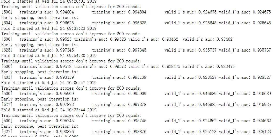

At the time of final submission, give me a surprise of 0.9430, a little wonder why the score is higher than the local training accuracy? Are some features not helpful in local training but effective in predicting? For the time being, if I drop 10%, I'm thinking about stacking several models (this method is hardly useful in production, but it's a big killer in competition, but I still hope to find more features and get better scores with the way out).