LightGBM is a fast, distributed and high performance gradient lifting framework based on decision tree algorithm. It can be used in sorting, classification, regression and many other machine learning tasks.
In the contest questions, we know that XGBoost algorithm is very popular, it is an excellent pull framework, but in the process of using, its training time is very long, and the memory occupation is relatively large. In January 2017, Microsoft opened a new boost tool, LightGBM, on GitHub. Without reducing the accuracy, the speed is increased by about 10 times and the occupied memory is reduced by about 3 times. Because it is based on decision tree algorithm, it uses optimal leaf wisdom strategy to split leaf nodes. However, other lifting algorithms usually use depth direction or level wisdom instead of leaf wisdom, which is wise. Therefore, in LightGBM algorithm, when growing to the same leaf nodes, Ye Min algorithm reduces more losses than horizontal-wise algorithm. As a result, it leads to higher accuracy, which can not be achieved by any other existing lifting algorithms.
In January 2017, Microsoft released its first stable version of LightGBM.
In the "Introduction to LightGBM" of AI headline sharing of Microsoft Asia Research Institute, Wang Taifeng, the lead researcher of Machine Learning Group, mentioned that after Microsoft DMTK team opened source on github and outperformed other decision tree tools LightGBM, it starred 1000 + times and forked more than 200 times in three days. Almost a thousand people are concerned about "How to view Microsoft's Open Source LightGBM?" Questions were rated as "amazing speed", "very enlightening", "supporting distributed", "clear and understandable code", "occupying little memory" and so on. The following are the various advantages of LightGBM that Microsoft officially mentioned, as well as the open source address of the project. Popular Science Link: How to Play LightGBM https://v.qq.com/x/page/k0362z6lqix.html
Catalog
Preface
What We Do in LightGBM?
Comparisons on Different Data Sets
3. Detailed Technology of LightGBM
1. Histogram optimization
2. Storage memory optimization
3. Depth-constrained Node Expansion Method
4. Histogram error optimization
5. Sequential Access Gradient
6. Supporting Category Characteristics
7. Supporting Parallel Learning
5. Implementation of LightGBM algorithm with python
What We Do in LightGBM?
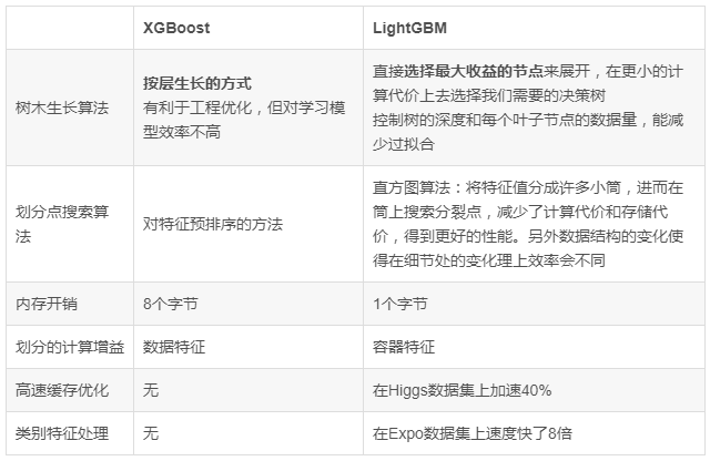
The table below gives a more detailed performance comparison between XGBoost and LightGBM, including the tree growth mode. LightGBM is directly to select the node to maximize the benefits, while XGBoost is done by layer-by-layer growth. LightGBM can build the decision tree we need at a lower computational cost. Of course, in such an algorithm, we also need to control the depth of the tree and the minimum amount of data for each leaf node, so as to reduce over-fitting.

Comparisons on Different Data Sets
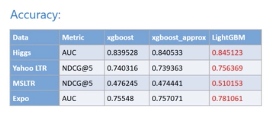
higgs and expo are categorized data, yahoo ltr and msltr are sorted data, in which LightGBM has better accuracy and stronger memory usage.

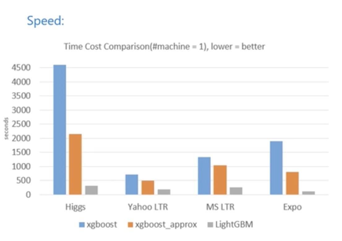
Comparing the computational speed, XGBoost usually takes more than several times as long to complete the same amount of training as LightGBM, and the gap between them is more than 15 times on the higgs data set.
3. Detailed Technology of LightGBM
1. Histogram optimization
In XGBoost, the method of pre-sorting is used. In the process of calculation, the dividing revenue is calculated according to the value order and the data samples one by one. Such an algorithm can find the best dividing value accurately, but the cost is relatively large and it has no good generalization.
In LightGBM, instead of using the traditional pre-ordering idea, these precise successive values are divided into a series of discrete domains, i.e. in the cylinder. Taking floating-point data as an example, the values of an interval are treated as barrels, and then the histograms of these barrels are used as units of accuracy. In this way, the expression of data becomes simpler, the use of memory is reduced, and the histogram brings a certain regularization effect, which can make our model avoid over-fitting and have better generalization.
Look at the details of histogram optimization
As you can see, this is to index the "histogram" according to bin, so it does not need to sort by each "feature" or compare the values of different "features" one by one, which greatly reduces the computational complexity.
2. Storage memory optimization
When we use data bin to describe the characteristics of data, the changes are: first, we do not need to store the sequence of each sorted data like the pre-sorting algorithm, that is, the gray table in the following figure. In LightGBM, the computational cost of this part is 0; second, generally bin will be controlled in a relatively small range. So we can store it in smaller memory.
3. Depth-constrained Node Expansion Method
LightGBM uses the Leaf-wise method with depth constraints to improve model accuracy, which is more efficient than Level-wise in XGBoost. It can reduce the training error and get better accuracy. However, the use of Leaf-wise alone may lead to deeper trees, which may result in over-fitting on small data sets, so there is an additional depth limit on Leaf-wise.
4. Histogram error optimization
Histogram difference optimization can achieve twice the acceleration. Histogram on a leaf node can be observed, which can be obtained by subtracting the histogram of its father node from that of its brother node. According to this point, we can construct the histogram on the leaf nodes with small amount of data, and then use the histogram difference to get the histogram on the leaf nodes with large amount of data, so as to achieve the acceleration effect.
5. Sequential Access Gradient
Two frequent operations in the pre-sorting algorithm lead to cache-miss, i.e. cache disappearance (which has a great impact on speed, especially when the amount of data is large, sequential access is more than four times faster than random access).
Access to gradients: Gradients need to be used when calculating gain. For different features, the order of access gradients is different and random.
Access to index tables: The pre-sorting algorithm uses index tables with row number and leaf node number to prevent all features from being segmented when data is segmented. Like access gradient, all features are indexed by accessing the index table.
These two operations are random access, which will bring about a great decline in system performance.
The histogram algorithm used by LightGBM can solve this kind of problem very well. First. For gradient access, because there is no need to rank features and all features are accessed in the same way, only the order of gradient access needs to be reordered, and all features can access gradients continuously. And the histogram algorithm does not need to put the data id on the leaf node number (no index table, no cache disappearance problem)
6. Supporting Category Characteristics
Traditional machine learning generally can not support direct input category features. It needs to be transformed into multi-dimensional 0-1 features, which is inefficient both in space and time. LightGBM improves the speed by nearly 8 times by changing the decision rules of decision tree algorithm, directly supporting category features without transformation.
7. Supporting Parallel Learning
LightGBM natively supports parallel learning. At present, it supports two kinds of parallel learning: Featrue Parallelization and Data Parallelization. Another is Voting Parallelization.
The main idea of feature parallelism is to find the optimal segmentation points on different machines and different feature sets, and then synchronize the optimal segmentation points among machines.
Data parallelism allows different machines to construct histograms locally, then merge them globally, and finally find the optimal segmentation points on the merged histograms.
LightGBM optimizes both parallel methods.
In feature parallel algorithm, all data are saved locally to avoid the communication of data segmentation results.
Reduce scatter is used in data parallel to allocate the task of histogram merging to different machines, reduce communication and computation, and make use of histogram to do bad, further reduce the traffic by half.
Voting Parallelization further optimizes the communication cost in data parallelization, making the communication cost become constant level. When the amount of data is large, voting parallelism can achieve very good acceleration effect.
The following figure better illustrates the overall process of the above three kinds of parallel learning:
In histogram merging, communication costs are relatively high, and voting-based data parallelism can solve this problem well.
Incremental training python code
I think this code is on another computer. Let's wait for it. Monday code to improve... First, a brief introduction of what incremental training is, that is, he can not eat so much data at a time, memory will burst, but what to read, there is a streaming reading method, essentially an iterator.
Each time a part of the file is read to train the model and save the training results of the model; then another part of the file is read, and then the model is updated for training; all the data are read iteratively, and finally the training process of the whole file data is completed.
1. Streaming Reading of Files
def iter_minibatches(minibatch_size=1000):
    '''
	//iterator
	//Given a file stream (such as a large file), output the minibatch_size line at a time, and select the default line of 1k
	//Convert output to numpy output, return X, y
	'''
    X = []
    y = []
    cur_line_num = 0

    train_data, train_label, train_weight, test_data, test_label, test_file = load_data()
    train_data, train_label = shuffle(train_data, train_label, random_state=0)  # random_state=0 is used to record the scrambling position to ensure that each scrambling position remains unchanged.
    print(type(train_label), train_label)

    for data_x, label_y in zip(train_data, train_label):
        X.append(data_x)
        y.append(label_y)

        cur_line_num += 1
        if cur_line_num >= minibatch_size:
            X, y = np.array(X), np.array(y)  # Converting data to numpy array type and returning
            yield X, y
            X, y = [], []
            cur_line_num = 0
2. lightgbm (LGB) Incremental Training Process
def lightgbmTest():
    import lightgbm as lgb
    # The first step is to initialize the model as None and set the model parameters.
    gbm = None
    params = {
        'task': 'train',
        'application': 'regression',  # objective function
        'boosting_type': 'gbdt',  # Setting Upgrade Types
        'learning_rate': 0.01,  # Learning rate
        'num_leaves': 50,  # Number of leaf nodes
        'tree_learner': 'serial',
        'min_data_in_leaf': 100,
        'metric': ['l1', 'l2', 'rmse'],  # l1:mae, l2:mse  # Evaluation function
        'max_bin': 255,
        'num_trees': 300
    }

    # The second step is streaming data (100,000 at a time)
    minibatch_train_iterators = iter_minibatches(minibatch_size=10000)

    for i, (X_, y_) in enumerate(minibatch_train_iterators):
        # Create lgb datasets
        # y_ = list(map(float, y_))  # Convert numpy.ndarray to list

        X_train, X_test, y_train, y_test = train_test_split(X_, y_, test_size=0.1, random_state=0)
        y_train = y_train.ravel()
        lgb_train = lgb.Dataset(X_train, y_train)
        lgb_eval = lgb.Dataset(X_test, y_test, reference=lgb_train)

        # Step 3: Incremental Training Model
        # Emphasis is laid on incremental training through init_model and keep_training_booster parameters.
        gbm = lgb.train(params,
                        lgb_train,
                        num_boost_round=1000,
                        valid_sets=lgb_eval,
                        init_model=gbm,  # If gbm is not None, then it is on the basis of the last training.
                        # feature_name=x_cols,
                        early_stopping_rounds=10,
                        verbose_eval=False,
                        keep_training_booster=True)  # Incremental training

        print("{} time".format(i))  # Current Number
        # Output Model Assessment Score
        score_train = dict([(s[1], s[2]) for s in gbm.eval_train()])
        print('The score of the current model in the training set is: mae=%.4f, mse=%.4f, rmse=%.4f'
              % (score_train['l1'], score_train['l2'], score_train['rmse']))

    return gbm
3. lightgbm (LGB) Call Procedure and Save Training Result Model
    '''lightgbm Incremental training'''
    print('lightgbm Incremental training')
    train_data, train_label, train_weight, test_data, test_label, test_file = load_data()
    print(train_label.shape,train_data.shape)
    train_X, test_X, train_Y, test_Y = train_test_split(train_data, train_label, test_size=0.1, random_state=0)
    # train_X, train_Y = shuffle(train_data, train_label, random_state=0)  # random_state=0 is used to record the scrambling position to ensure that each scrambling position remains unchanged.

    gbm = lightgbmTest()
    pred_Y = gbm.predict(test_X)
    print('compute_loss:{}'.format(compute_loss(test_Y, pred_Y)))

    # gbm.save_model('lightgbmtest.model')
    # Model Storage
    joblib.dump(gbm, 'loan_model.pkl')
    # Model Loading
    gbm = joblib.load('loan_model.pkl')
Light GBM parametric adjustment method
In fact, for the model based on decision tree, the methods of parameter adjustment are similar to each other. Generally, the following steps are required:
-
First, choose a higher learning rate, about 0.1, in order to speed up the convergence rate. This is necessary for adjusting the parameters.
-
Adjusting the Basic Parameters of Decision Tree
-
Regularized parameter tuning
-
Finally, reduce the learning rate, here is to improve the accuracy of the final.
Therefore, the following parametric adjustment example is based on the above steps to operate. The data set is a (4400+, 1000+) data set, all of which are numerical features. The metric uses root mean square error.
(PS: or Tucao, there are too many synonyms (alias) of the lightgbm parameter. Sometimes different parameters are really troubled by the same meaning. I use the following synonymous parameters to make them easy to see.
Step1. Learning Rate and Estimator and Its Number
Anyway, let's take learning_rate = 0.1 first, and then determine the type of estimator boosting/boost/boosting_type, but gbdt will be chosen by default.
To determine the number of estimators, that is, the number of boosting iterations, or the number of residual trees, the parameter is n_estimators/num_iterations/num_round/num_boost_round. We can first set this parameter to a larger number, and then look at the optimal number of iterations in the cv results, such as the code.
Before that, we must give an initial value to other important parameters. The initial value is of little significance, just for the convenience of determining other parameters. Let's start with an initial value:
The following parameters are determined according to specific project requirements:
'boosting_type'/'boosting': 'gbdt''objective': 'regression''metric': 'rmse'
The following parameters I choose are the initial values, you can choose according to your own situation:
'max_depth': 6. \ Decide according to the question, because my data set is not very large, so choose a moderate value, in fact, 4-10 does not matter. 'num_leaves': 50 \ because lightGBM is grown by leaves_wise, the official saying is less than 2^max_depth'subsample'/'bagging_fraction':0.8 colsample_bytree'/'feature_fraction': 0.8 feature_fraction feature sampling
Next, I use LightGBM's cv function to demonstrate:
params = {    'boosting_type': 'gbdt',
    'objective': 'regression',

    'learning_rate': 0.1,
    'num_leaves': 50,
    'max_depth': 6,    'subsample': 0.8,
    'colsample_bytree': 0.8,
    }
data_train = lgb.Dataset(df_train, y_train, silent=True)
cv_results = lgb.cv(
params, data_train, num_boost_round=1000, nfold=5, stratified=False, shuffle=True, metrics='rmse',
early_stopping_rounds=50, verbose_eval=50, show_stdv=True, seed=0)
print('best n_estimators:', len(cv_results['rmse-mean']))
print('best cv score:', cv_results['rmse-mean'][-1])[50] cv_agg's rmse: 1.38497 + 0.0202823best n_estimators: 43best cv score: 1.3838664241
Because my data set is not very large, when the learning rate is 0.1, the optimal number of iterations is only 43. Now let's substitute (0.1, 43) into tuning for other parameters. However, it is suggested that the lower the learning rate, the better the hardware conditions permit.
Step2. max_depth and num_leaves
This is the most important parameter to improve accuracy.
max_depth: Setting tree depth, the greater the depth, the more likely it is to be over-fitting
Num_leaves: Because LightGBM uses the leaf-wise algorithm, it uses num_leaves instead of max_depth to adjust the complexity of the tree. Rough conversion relationship: num_leaves = 2^(max_depth), but its value should be set less than 2^(max_depth), otherwise it may lead to over-fitting.
We can also adjust these two parameters at the same time. For these two parameters, we first roughly adjust, then fine-tune.
Here we introduce the GridSearchCV() function in sklearn s to search. Somehow, this function consumes memory, time and energy.
from sklearn.model_selection import GridSearchCV###We can create a sklearn er model of lgb, using the model_lgb = lgb.LGBMRegressor(objective='regression',num_leaves=50) selected above.
                              learning_rate=0.1, n_estimators=43, max_depth=6,
                              metric='rmse', bagging_fraction = 0.8,feature_fraction = 0.8)

params_test1={    'max_depth': range(3,8,2),    'num_leaves':range(50, 170, 30)
}
gsearch1 = GridSearchCV(estimator=model_lgb, param_grid=params_test1, scoring='neg_mean_squared_error', cv=5, verbose=1, n_jobs=4)
gsearch1.fit(df_train, y_train) gsearch1.grid_scores_, gsearch1.best_params_, gsearch1.best_score_
Fitting 5 folds for each of 12 candidates, totalling 60 fits


[Parallel(n_jobs=4)]: Done  42 tasks      | elapsed:  2.0min
[Parallel(n_jobs=4)]: Done  60 out of  60 | elapsed:  3.1min finished


([mean: -1.88629, std: 0.13750, params: {'max_depth': 3, 'num_leaves': 50},  mean: -1.88629, std: 0.13750, params: {'max_depth': 3, 'num_leaves': 80},  mean: -1.88629, std: 0.13750, params: {'max_depth': 3, 'num_leaves': 110},  mean: -1.88629, std: 0.13750, params: {'max_depth': 3, 'num_leaves': 140},  mean: -1.86917, std: 0.12590, params: {'max_depth': 5, 'num_leaves': 50},  mean: -1.86917, std: 0.12590, params: {'max_depth': 5, 'num_leaves': 80},  mean: -1.86917, std: 0.12590, params: {'max_depth': 5, 'num_leaves': 110},  mean: -1.86917, std: 0.12590, params: {'max_depth': 5, 'num_leaves': 140},  mean: -1.89254, std: 0.10904, params: {'max_depth': 7, 'num_leaves': 50},  mean: -1.86024, std: 0.11364, params: {'max_depth': 7, 'num_leaves': 80},  mean: -1.86024, std: 0.11364, params: {'max_depth': 7, 'num_leaves': 110},  mean: -1.86024, std: 0.11364, params: {'max_depth': 7, 'num_leaves': 140}],
 {'max_depth': 7, 'num_leaves': 80}, -1.8602436718814157)
Here, we run 12 parameter combinations, and the optimal solution is - 1.860 with max_depth of 7 and num_leaves of 80.
It must be said here that the scoring parameters in sklearn model evaluation are higher return values are better than lower return values (higher return values are better than lower return values).
However, the metric strategy I used was rmse, the lower the better, so sklearn s provided neg_mean_squared_erro parameter, that is, the negative number of metrics returned, so in terms of mean square deviation, the larger the negative number, the better.
Therefore, we can see that the score of the optimal solution is -1.860, which is translated into np. sqrt (-(-1.860))= 1.3639, which is much better than that of step 1.
At this point, we replace the optimal solution obtained by this step with the third step. In fact, I have only made a rough adjustment here. If we want to get a better result, we can take a few more values near 7 for max_depth and a few more values near 80 for num_leaves. Don't be afraid of trouble, although it's really troublesome.
params_test2={    'max_depth': [6,7,8],    'num_leaves':[68,74,80,86,92]
}

gsearch2 = GridSearchCV(estimator=model_lgb, param_grid=params_test2, scoring='neg_mean_squared_error', cv=5, verbose=1, n_jobs=4)
gsearch2.fit(df_train, y_train)
gsearch2.grid_scores_, gsearch2.best_params_, gsearch2.best_score_
Fitting 5 folds for each of 15 candidates, totalling 75 fits
[Parallel(n_jobs=4)]: Done 42 tasks | elapsed: 2.8min
[Parallel(n_jobs=4)]: Done 75 out of 75 | elapsed: 5.1min finished
([mean: -1.87506, std: 0.11369, params: {'max_depth': 6, 'num_leaves': 68}, mean: -1.87506, std: 0.11369, params: {'max_depth': 6, 'num_leaves': 74}, mean: -1.87506, std: 0.11369, params: {'max_depth': 6, 'num_leaves': 80}, mean: -1.87506, std: 0.11369, params: {'max_depth': 6, 'num_leaves': 86}, mean: -1.87506, std: 0.11369, params: {'max_depth': 6, 'num_leaves': 92}, mean: -1.86024, std: 0.11364, params: {'max_depth': 7, 'num_leaves': 68}, mean: -1.86024, std: 0.11364, params: {'max_depth': 7, 'num_leaves': 74}, mean: -1.86024, std: 0.11364, params: {'max_depth': 7, 'num_leaves': 80}, mean: -1.86024, std: 0.11364, params: {'max_depth': 7, 'num_leaves': 86}, mean: -1.86024, std: 0.11364, params: {'max_depth': 7, 'num_leaves': 92}, mean: -1.88197, std: 0.11295, params: {'max_depth': 8, 'num_leaves': 68}, mean: -1.89117, std: 0.12686, params: {'max_depth': 8, 'num_leaves': 74}, mean: -1.86390, std: 0.12259, params: {'max_depth': 8, 'num_leaves': 80}, mean: -1.86733, std: 0.12159, params: {'max_depth': 8, 'num_leaves': 86}, mean: -1.86665, std: 0.12174, params: {'max_depth': 8, 'num_leaves': 92}],
{'max_depth': 7, 'num_leaves': 68}, -1.8602436718814157)It can be seen that the maximum depth of 7 is no problem, but if you look at the details, it is found that the number of leaf nodes has no effect on the score when the maximum depth is 7.
Step3: min_data_in_leaf and min_sum_hessian_in_leaf
At this point, it's time to reduce the over-fitting.
min_data_in_leaf is an important parameter, also known as min_child_samples. Its value depends on the sample tree and num_leaves of training data. Setting it larger can avoid generating a deep tree, but it may lead to underfitting.
min_sum_hessian_in_leaf: also known as min_child_weight, the sum of the minimum Heisen values that divide a node, is a minimum sum of Hessians in one leaf to allow a split. Higher values are reduced overfitting.
We adopt the same method as above:
params_test3={    'min_child_samples': [18, 19, 20, 21, 22],    'min_child_weight':[0.001, 0.002]
}
model_lgb = lgb.LGBMRegressor(objective='regression',num_leaves=80,
                              learning_rate=0.1, n_estimators=43, max_depth=7,
                              metric='rmse', bagging_fraction = 0.8, feature_fraction = 0.8)
gsearch3 = GridSearchCV(estimator=model_lgb, param_grid=params_test3, scoring='neg_mean_squared_error', cv=5, verbose=1, n_jobs=4)
gsearch3.fit(df_train, y_train)
gsearch3.grid_scores_, gsearch3.best_params_, gsearch3.best_score_
Fitting 5 folds for each of 10 candidates, totalling 50 fits
[Parallel(n_jobs=4)]: Done 42 tasks | elapsed: 2.9min
[Parallel(n_jobs=4)]: Done 50 out of 50 | elapsed: 3.3min finished
([mean: -1.88057, std: 0.13948, params: {'min_child_samples': 18, 'min_child_weight': 0.001}, mean: -1.88057, std: 0.13948, params: {'min_child_samples': 18, 'min_child_weight': 0.002}, mean: -1.88365, std: 0.13650, params: {'min_child_samples': 19, 'min_child_weight': 0.001}, mean: -1.88365, std: 0.13650, params: {'min_child_samples': 19, 'min_child_weight': 0.002}, mean: -1.86024, std: 0.11364, params: {'min_child_samples': 20, 'min_child_weight': 0.001}, mean: -1.86024, std: 0.11364, params: {'min_child_samples': 20, 'min_child_weight': 0.002}, mean: -1.86980, std: 0.14251, params: {'min_child_samples': 21, 'min_child_weight': 0.001}, mean: -1.86980, std: 0.14251, params: {'min_child_samples': 21, 'min_child_weight': 0.002}, mean: -1.86750, std: 0.13898, params: {'min_child_samples': 22, 'min_child_weight': 0.001}, mean: -1.86750, std: 0.13898, params: {'min_child_samples': 22, 'min_child_weight': 0.002}],
{'min_child_samples': 20, 'min_child_weight': 0.001}, -1.8602436718814157)This is the result of fine tuning after rough tuning. It can be seen that the optimal value of min_data_in_leaf is 20, while min_sum_hessian_in_leaf has little effect on the final value. And after adjusting parameters here, the final value is not optimized, indicating that the default value before is 20,0.001.
Step4: feature_fraction and bagging_fraction
Both parameters are designed to reduce over-fitting.
The feature_fraction parameter is used for feature subsampling. This parameter can be used to prevent over-fitting and improve training speed.
The parameters of bagging_fraction+bagging_freq must be set at the same time. Bagging_fraction is equivalent to subsample sample sampling, which can make bagging run faster and reduce fitting. Bagging_freq defaults to 0, indicating the frequency of bagging. 0 means that bagging is not used, and k means bagging once per k iteration.
Different parameters, the same method.
params_test4={    'feature_fraction': [0.5, 0.6, 0.7, 0.8, 0.9],    'bagging_fraction': [0.6, 0.7, 0.8, 0.9, 1.0]
}
model_lgb = lgb.LGBMRegressor(objective='regression',num_leaves=80,
                              learning_rate=0.1, n_estimators=43, max_depth=7,
                              metric='rmse', bagging_freq = 5,  min_child_samples=20)
gsearch4 = GridSearchCV(estimator=model_lgb, param_grid=params_test4, scoring='neg_mean_squared_error', cv=5, verbose=1, n_jobs=4)
gsearch4.fit(df_train, y_train)
gsearch4.grid_scores_, gsearch4.best_params_, gsearch4.best_score_
Fitting 5 folds for each of 25 candidates, totalling 125 fits
[Parallel(n_jobs=4)]: Done 42 tasks | elapsed: 2.6min
[Parallel(n_jobs=4)]: Done 125 out of 125 | elapsed: 7.1min finished
([mean: -1.90447, std: 0.15841, params: {'bagging_fraction': 0.6, 'feature_fraction': 0.5}, mean: -1.90846, std: 0.13925, params: {'bagging_fraction': 0.6, 'feature_fraction': 0.6}, mean: -1.91695, std: 0.14121, params: {'bagging_fraction': 0.6, 'feature_fraction': 0.7}, mean: -1.90115, std: 0.12625, params: {'bagging_fraction': 0.6, 'feature_fraction': 0.8}, mean: -1.92586, std: 0.15220, params: {'bagging_fraction': 0.6, 'feature_fraction': 0.9}, mean: -1.88031, std: 0.17157, params: {'bagging_fraction': 0.7, 'feature_fraction': 0.5}, mean: -1.89513, std: 0.13718, params: {'bagging_fraction': 0.7, 'feature_fraction': 0.6}, mean: -1.88845, std: 0.13864, params: {'bagging_fraction': 0.7, 'feature_fraction': 0.7}, mean: -1.89297, std: 0.12374, params: {'bagging_fraction': 0.7, 'feature_fraction': 0.8}, mean: -1.89432, std: 0.14353, params: {'bagging_fraction': 0.7, 'feature_fraction': 0.9}, mean: -1.88088, std: 0.14247, params: {'bagging_fraction': 0.8, 'feature_fraction': 0.5}, mean: -1.90080, std: 0.13174, params: {'bagging_fraction': 0.8, 'feature_fraction': 0.6}, mean: -1.88364, std: 0.14732, params: {'bagging_fraction': 0.8, 'feature_fraction': 0.7}, mean: -1.88987, std: 0.13344, params: {'bagging_fraction': 0.8, 'feature_fraction': 0.8}, mean: -1.87752, std: 0.14802, params: {'bagging_fraction': 0.8, 'feature_fraction': 0.9}, mean: -1.88348, std: 0.13925, params: {'bagging_fraction': 0.9, 'feature_fraction': 0.5}, mean: -1.87472, std: 0.13301, params: {'bagging_fraction': 0.9, 'feature_fraction': 0.6}, mean: -1.88656, std: 0.12241, params: {'bagging_fraction': 0.9, 'feature_fraction': 0.7}, mean: -1.89029, std: 0.10776, params: {'bagging_fraction': 0.9, 'feature_fraction': 0.8}, mean: -1.88719, std: 0.11915, params: {'bagging_fraction': 0.9, 'feature_fraction': 0.9}, mean: -1.86170, std: 0.12544, params: {'bagging_fraction': 1.0, 'feature_fraction': 0.5}, mean: -1.87334, std: 0.13099, params: {'bagging_fraction': 1.0, 'feature_fraction': 0.6}, mean: -1.85412, std: 0.12698, params: {'bagging_fraction': 1.0, 'feature_fraction': 0.7}, mean: -1.86024, std: 0.11364, params: {'bagging_fraction': 1.0, 'feature_fraction': 0.8}, mean: -1.87266, std: 0.12271, params: {'bagging_fraction': 1.0, 'feature_fraction': 0.9}],
{'bagging_fraction': 1.0, 'feature_fraction': 0.7}, -1.8541224387666373)It can be seen from this that the ideal values of bagging_feature and feature_fraction are 1.0 and 0.7 respectively. One important reason is that my sample size is relatively small (4000+), but the number of features is very large (1000+). So, here we take a smaller step and take a more detailed value of feature_fraction.
params_test5={    'feature_fraction': [0.62, 0.65, 0.68, 0.7, 0.72, 0.75, 0.78 ]
}
model_lgb = lgb.LGBMRegressor(objective='regression',num_leaves=80,
                              learning_rate=0.1, n_estimators=43, max_depth=7,
                              metric='rmse',  min_child_samples=20)
gsearch5 = GridSearchCV(estimator=model_lgb, param_grid=params_test5, scoring='neg_mean_squared_error', cv=5, verbose=1, n_jobs=4)
gsearch5.fit(df_train, y_train)
gsearch5.grid_scores_, gsearch5.best_params_, gsearch5.best_score_
Fitting 5 folds for each of 7 candidates, totalling 35 fits
[Parallel(n_jobs=4)]: Done 35 out of 35 | elapsed: 2.3min finished
([mean: -1.86696, std: 0.12658, params: {'feature_fraction': 0.62}, mean: -1.88337, std: 0.13215, params: {'feature_fraction': 0.65}, mean: -1.87282, std: 0.13193, params: {'feature_fraction': 0.68}, mean: -1.85412, std: 0.12698, params: {'feature_fraction': 0.7}, mean: -1.88235, std: 0.12682, params: {'feature_fraction': 0.72}, mean: -1.86329, std: 0.12757, params: {'feature_fraction': 0.75}, mean: -1.87943, std: 0.12107, params: {'feature_fraction': 0.78}],
{'feature_fraction': 0.7}, -1.8541224387666373)Well, feature_fraction is 0.7.
Step5: Regularization parameter
The regularization parameters lambda_l1 (reg_alpha) and lambda_l2 (reg_lambda) undoubtedly reduce the over-fitting. They correspond to L1 regularization and L2 regularization respectively. Let's also try to use these two parameters.
params_test6={    'reg_alpha': [0, 0.001, 0.01, 0.03, 0.08, 0.3, 0.5],    'reg_lambda': [0, 0.001, 0.01, 0.03, 0.08, 0.3, 0.5]
}
model_lgb = lgb.LGBMRegressor(objective='regression',num_leaves=80,
                              learning_rate=0.b1, n_estimators=43, max_depth=7,
                              metric='rmse',  min_child_samples=20, feature_fraction=0.7)
gsearch6 = GridSearchCV(estimator=model_lgb, param_grid=params_test6, scoring='neg_mean_squared_error', cv=5, verbose=1, n_jobs=4)
gsearch6.fit(df_train, y_train)
gsearch6.grid_scores_, gsearch6.best_params_, gsearch6.best_score_
Fitting 5 folds for each of 49 candidates, totalling 245 fits
[Parallel(n_jobs=4)]: Done 42 tasks | elapsed: 2.8min
[Parallel(n_jobs=4)]: Done 192 tasks | elapsed: 10.6min
[Parallel(n_jobs=4)]: Done 245 out of 245 | elapsed: 13.3min finished
([mean: -1.85412, std: 0.12698, params: {'reg_alpha': 0, 'reg_lambda': 0}, mean: -1.85990, std: 0.13296, params: {'reg_alpha': 0, 'reg_lambda': 0.001}, mean: -1.86367, std: 0.13634, params: {'reg_alpha': 0, 'reg_lambda': 0.01}, mean: -1.86787, std: 0.13881, params: {'reg_alpha': 0, 'reg_lambda': 0.03}, mean: -1.87099, std: 0.12476, params: {'reg_alpha': 0, 'reg_lambda': 0.08}, mean: -1.87670, std: 0.11849, params: {'reg_alpha': 0, 'reg_lambda': 0.3}, mean: -1.88278, std: 0.13064, params: {'reg_alpha': 0, 'reg_lambda': 0.5}, mean: -1.86190, std: 0.13613, params: {'reg_alpha': 0.001, 'reg_lambda': 0}, mean: -1.86190, std: 0.13613, params: {'reg_alpha': 0.001, 'reg_lambda': 0.001}, mean: -1.86515, std: 0.14116, params: {'reg_alpha': 0.001, 'reg_lambda': 0.01}, mean: -1.86908, std: 0.13668, params: {'reg_alpha': 0.001, 'reg_lambda': 0.03}, mean: -1.86852, std: 0.12289, params: {'reg_alpha': 0.001, 'reg_lambda': 0.08}, mean: -1.88076, std: 0.11710, params: {'reg_alpha': 0.001, 'reg_lambda': 0.3}, mean: -1.88278, std: 0.13064, params: {'reg_alpha': 0.001, 'reg_lambda': 0.5}, mean: -1.87480, std: 0.13889, params: {'reg_alpha': 0.01, 'reg_lambda': 0}, mean: -1.87284, std: 0.14138, params: {'reg_alpha': 0.01, 'reg_lambda': 0.001}, mean: -1.86030, std: 0.13332, params: {'reg_alpha': 0.01, 'reg_lambda': 0.01}, mean: -1.86695, std: 0.12587, params: {'reg_alpha': 0.01, 'reg_lambda': 0.03}, mean: -1.87415, std: 0.13100, params: {'reg_alpha': 0.01, 'reg_lambda': 0.08}, mean: -1.88543, std: 0.13195, params: {'reg_alpha': 0.01, 'reg_lambda': 0.3}, mean: -1.88076, std: 0.13502, params: {'reg_alpha': 0.01, 'reg_lambda': 0.5}, mean: -1.87729, std: 0.12533, params: {'reg_alpha': 0.03, 'reg_lambda': 0}, mean: -1.87435, std: 0.12034, params: {'reg_alpha': 0.03, 'reg_lambda': 0.001}, mean: -1.87513, std: 0.12579, params: {'reg_alpha': 0.03, 'reg_lambda': 0.01}, mean: -1.88116, std: 0.12218, params: {'reg_alpha': 0.03, 'reg_lambda': 0.03}, mean: -1.88052, std: 0.13585, params: {'reg_alpha': 0.03, 'reg_lambda': 0.08}, mean: -1.87565, std: 0.12200, params: {'reg_alpha': 0.03, 'reg_lambda': 0.3}, mean: -1.87935, std: 0.13817, params: {'reg_alpha': 0.03, 'reg_lambda': 0.5}, mean: -1.87774, std: 0.12477, params: {'reg_alpha': 0.08, 'reg_lambda': 0}, mean: -1.87774, std: 0.12477, params: {'reg_alpha': 0.08, 'reg_lambda': 0.001}, mean: -1.87911, std: 0.12027, params: {'reg_alpha': 0.08, 'reg_lambda': 0.01}, mean: -1.86978, std: 0.12478, params: {'reg_alpha': 0.08, 'reg_lambda': 0.03}, mean: -1.87217, std: 0.12159, params: {'reg_alpha': 0.08, 'reg_lambda': 0.08}, mean: -1.87573, std: 0.14137, params: {'reg_alpha': 0.08, 'reg_lambda': 0.3}, mean: -1.85969, std: 0.13109, params: {'reg_alpha': 0.08, 'reg_lambda': 0.5}, mean: -1.87632, std: 0.12398, params: {'reg_alpha': 0.3, 'reg_lambda': 0}, mean: -1.86995, std: 0.12651, params: {'reg_alpha': 0.3, 'reg_lambda': 0.001}, mean: -1.86380, std: 0.12793, params: {'reg_alpha': 0.3, 'reg_lambda': 0.01}, mean: -1.87577, std: 0.13002, params: {'reg_alpha': 0.3, 'reg_lambda': 0.03}, mean: -1.87402, std: 0.13496, params: {'reg_alpha': 0.3, 'reg_lambda': 0.08}, mean: -1.87032, std: 0.12504, params: {'reg_alpha': 0.3, 'reg_lambda': 0.3}, mean: -1.88329, std: 0.13237, params: {'reg_alpha': 0.3, 'reg_lambda': 0.5}, mean: -1.87196, std: 0.13099, params: {'reg_alpha': 0.5, 'reg_lambda': 0}, mean: -1.87196, std: 0.13099, params: {'reg_alpha': 0.5, 'reg_lambda': 0.001}, mean: -1.88222, std: 0.14735, params: {'reg_alpha': 0.5, 'reg_lambda': 0.01}, mean: -1.86618, std: 0.14006, params: {'reg_alpha': 0.5, 'reg_lambda': 0.03}, mean: -1.88579, std: 0.12398, params: {'reg_alpha': 0.5, 'reg_lambda': 0.08}, mean: -1.88297, std: 0.12307, params: {'reg_alpha': 0.5, 'reg_lambda': 0.3}, mean: -1.88148, std: 0.12622, params: {'reg_alpha': 0.5, 'reg_lambda': 0.5}],
{'reg_alpha': 0, 'reg_lambda': 0}, -1.8541224387666373)Ha-ha, it seems that I've done too much.
Step 6: Reduce learning_rate
Previous use of higher learning rate is because it can make convergence faster, but the accuracy is certainly not as good as the long flow of water. Finally, we use a lower learning rate and more decision tree n_estimators to train the data to see if we can further optimize the score.
We can use the cv function of lightGBM again, and we can substitute the parameters we optimized before.
params = {    'boosting_type': 'gbdt',
    'objective': 'regression',

    'learning_rate': 0.005,
    'num_leaves': 80,
    'max_depth': 7,    'min_data_in_leaf': 20,    'subsample': 1,
    'colsample_bytree': 0.7,
    }

data_train = lgb.Dataset(df_train, y_train, silent=True)
cv_results = lgb.cv(
    params, data_train, num_boost_round=10000, nfold=5, stratified=False, shuffle=True, metrics='rmse',
    early_stopping_rounds=50, verbose_eval=100, show_stdv=True)

print('best n_estimators:', len(cv_results['rmse-mean']))
print('best cv score:', cv_results['rmse-mean'][-1])
This is a general process, in fact, there are more advanced methods, but this basic GBM model parameter adjustment method also needs to be understood. If you have any questions, please give more advice.