Gradually Establishing Deep Neural Networks

Welcome to your fourth week assignment (Part 1, Part 2)! You have trained a two-layer neural network (with only one hidden layer). This week, you'll build a deep neural network, and you'll have as many layers as you want!

In this section, you will implement all the functions required to build deep neural networks. In the next assignment, you will use these functions to build a deep neural network for image classification. After completing this task, you will be able to:

• Improving the model by using non-linear elements such as ReLU
• Establish a deeper neural network (with more than one hidden layer)
• Implementing an Easy-to-Use Class of Neural Networks

1 - Preparing software packages

Let's first import all the packages you need for this task.

• numpy: It's the main software package for scientific computing using Python.
• matplotlib: It's a library of graphics drawn with Python.
• dnn_utils: This notebook provides some necessary functions.
• Test cases: Provide some test cases to evaluate the correctness of your functions
• np.random.seed(1): Used to maintain the consistency of all random function calls. This will help us to grade your work. Please don't change seeds.

import numpy as np
import h5py
import matplotlib.pyplot as plt
from testCases_v2 import *
from dnn_utils_v2 import sigmoid, sigmoid_backward, relu, relu_backward

%matplotlib inline
plt.rcParams['figure.figsize'] = (5.0, 4.0) # set default size of plots
plt.rcParams['image.interpolation'] = 'nearest'
plt.rcParams['image.cmap'] = 'gray'

%load_ext autoreload
%autoreload 2

np.random.seed(1)

 

2 - Operational Outline

In order to build your neural network, you will implement several "help functions". These auxiliary functions will be used in the next task to construct a two-layer neural network and an L-layer neural network. Each help function you will implement will be described in detail to guide you through the necessary steps. Following is the outline of this assignment. You will:

• Initialize the parameters of two-layer network and one-layer neural network.
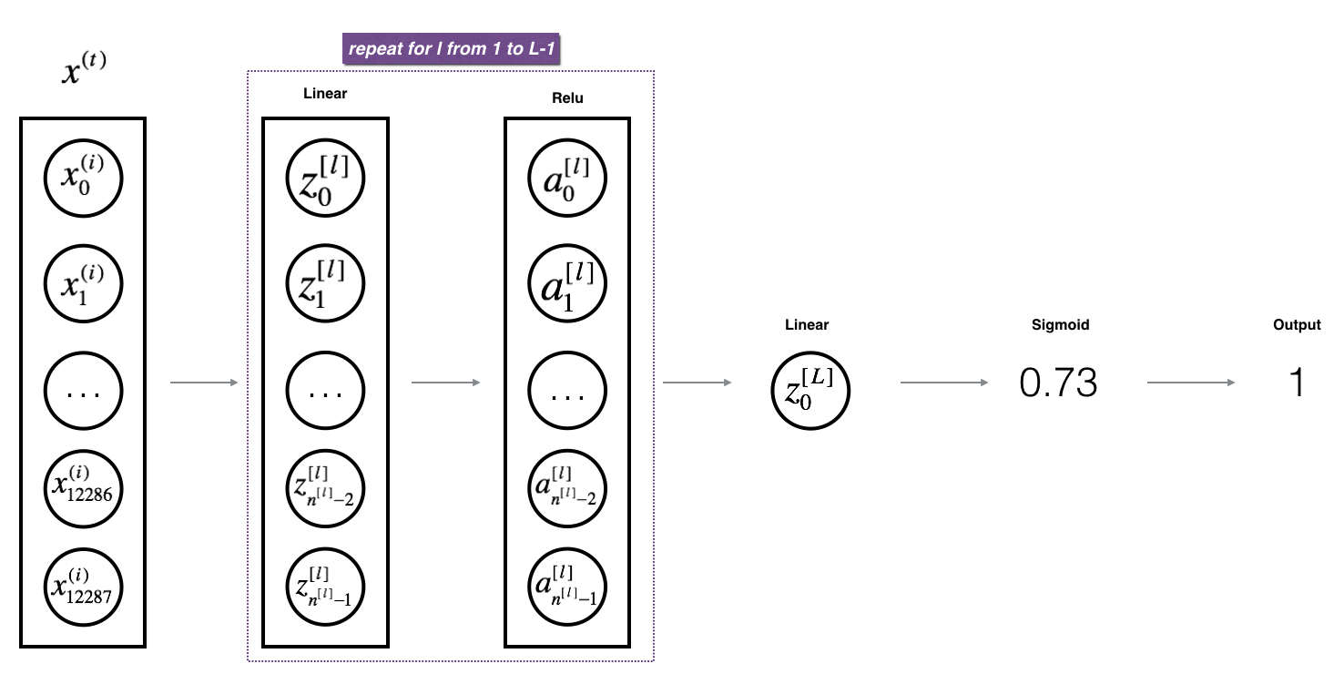
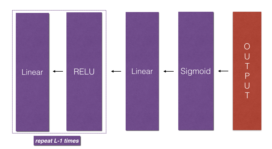
• Implement forward propagation module (shown in purple in the figure below).
• Complete the linear part of the forward propagation step of the layer (the result is in Z[l].
• Let's give you the activation function (relu/sigmoid).
• Combine the first two steps into a new [LINEAR - > ACTIVATION] forward function.
• Stack [LINEAR - > ACTIVATION] forward function L-1 once (for Layers 1 to L-1) and add a [LINEAR - > SIGMOID] at the end (for Layers 1 to L-1). This gives you a new L_model_forward function.
• Calculate the loss.
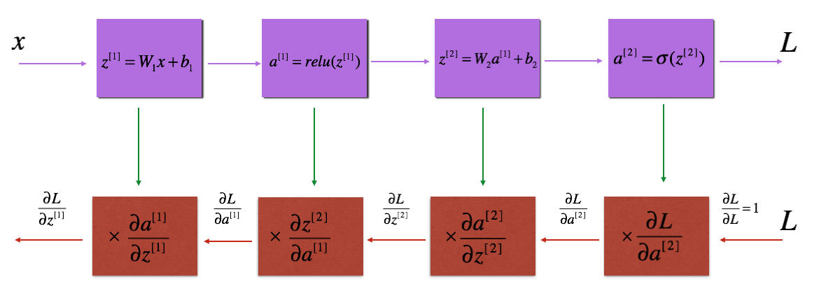
• Implement the back propagation module (shown in red in the figure below).
• Complete the linear part of the layer back propagation step.
• We give you the gradient of the activation function (relu_backward/sigmoid_backward)
• Combine the first two steps into a new [LINEAR - > ACTIVATION] backward function.
• Stack [LINEAR-> RELU] backward function L-1 times and add [LINEAR-> SIGMOID] backward in the new L_model_backward function
• Finally, the parameters are updated.

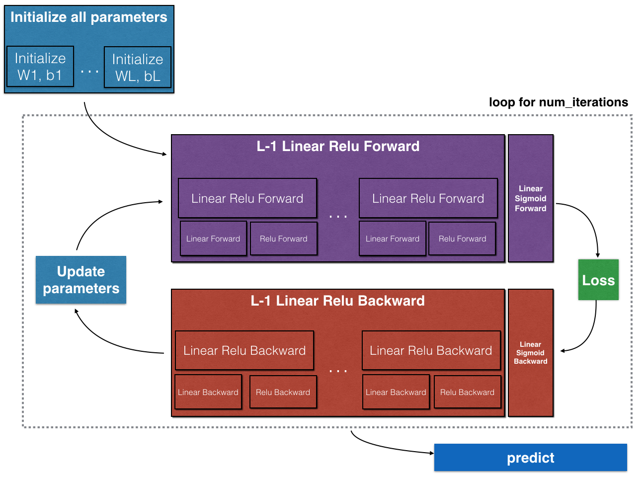
Note that for each forward function, there is a corresponding reverse function. That's why at every step of the forwarding module, you store some values in the cache. Cached values are useful for calculating gradients. In the reverse propagation module, you will use the cache to calculate the gradient. This assignment will show you how to perform these steps.

 

3 - Initialization parameters

You will write two help functions to initialize the parameters of the model. The first function will be used to initialize the parameters of the two-tier model. The second one will extend the initialization process to L layer.

3.1-Two-Layer Neural Network

Exercise: Create and initialize parameters of two-layer neural network.

Explain:

• The structure of the model is linear - > ReLU - > linear - > SIGMOD function.
• The weight matrix is initialized randomly. Use the correct latitude np.random.randn(shape)*0.01.
• Use zero initialization for bias. Use np.zeros(shape).

# GRADED FUNCTION: initialize_parameters

def initialize_parameters(n_x, n_h, n_y):
    """
    //This function is used to initialize two-layer network parameters.
    //Parameters:
        n_x - Number of input layer nodes
        n_h - Number of Hidden Layer Nodes
        n_y - Number of Output Layer Nodes

    //Return:
        parameters - Including your parameters python Dictionaries:
            W1 - Weight Matrix,Dimensions are( n_h，n_x)
            b1 - Partial vector, dimension( n_h，1)
            W2 - Weight matrix, dimension is( n_y，n_h)
            b2 - Partial vector, dimension( n_y，1)
    """
    
    np.random.seed(1)
    
    ### START CODE HERE ### (≈ 4 lines of code)
    W1 = np.random.randn(n_h, n_x) * 0.01
    b1 = np.zeros((n_h, 1))
    W2 = np.random.randn(n_y, n_h) * 0.01
    b2 = np.zeros((n_y, 1))
    ### END CODE HERE ###
    
    # Use assertions to ensure that my data format is correct
    assert(W1.shape == (n_h, n_x))
    assert(b1.shape == (n_h, 1))
    assert(W2.shape == (n_y, n_h))
    assert(b2.shape == (n_y, 1))
    
    parameters = {"W1": W1,
                  "b1": b1,
                  "W2": W2,
                  "b2": b2}
    
    return parameters    

Test:

parameters = initialize_parameters(2,2,1)
print("W1 = " + str(parameters["W1"]))
print("b1 = " + str(parameters["b1"]))
print("W2 = " + str(parameters["W2"]))
print("b2 = " + str(parameters["b2"]))

Result:

W1 = [[ 0.01624345 -0.00611756]
 [-0.00528172 -0.01072969]]
b1 = [[0.]
 [0.]]
W2 = [[ 0.00865408 -0.02301539]]
b2 = [[0.]]

 

3.2-L Layer Neural Network

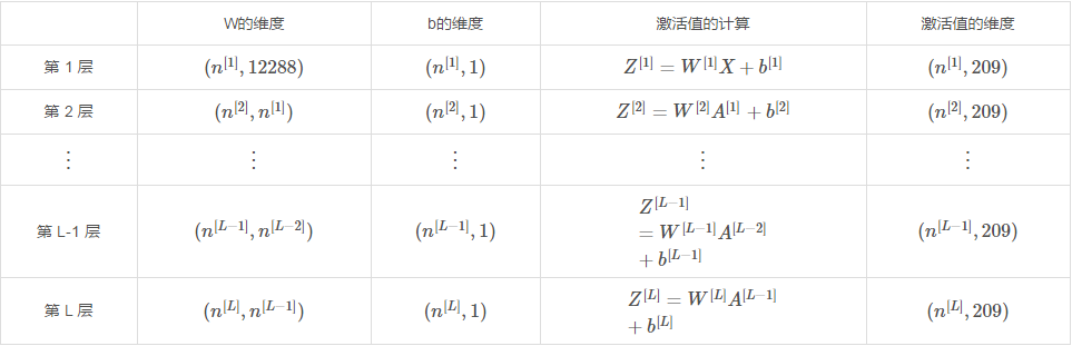
Initialization of deeper L-layer neural networks is more complex because there are more weight matrices and bias vectors. When initialize_parameters_deep is completed, you should ensure that the dimensions of each layer match. Recall that n[l] is the unit in layer L. Assume that the dimension of X (input data) is (12288, 209) (m=209 examples):

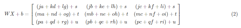
Remember, when we calculate + WX+b with python, it performs broadcasting. For example, if:

Then WX+b will be:

 

Exercise: Implement the initialization of an L-layer neural network.

Explain:

• The structure of the model is [LINEAR-> RELU] * L-1-> LINEAR-> SIGMOID. I.e. It has an L-1 layer using the ReLU activation function, followed by an output layer with the sigmoid activation function.
• The weight matrix is initialized randomly and np.random.rand(shape)* 0.01 is used.
• Zero initialization is used for bias and np.zeros(shape) is used.
• We will store n[l], the units in different layers, in a variable layer_dims. For example, the layer_dims of last week's "plane data classification model" should be [2, 4, 1]: there are two inputs, one hidden layer has four hidden units, and one output layer has one output unit. So it means that the dimension of W1 is (4,2), b1 is (4,1), W2 is (1,4), and b2 is (1,1). Now you're going to extend it to Layer L!
• The following is the implementation of L=1 (single layer neural network). It should motivate you to implement the general situation (L-layer neural network).

if L == 1:
      parameters["W" + str(L)] = np.random.randn(layer_dims[1], layer_dims[0]) * 0.01
      parameters["b" + str(L)] = np.zeros((layer_dims[1], 1))

# GRADED FUNCTION: initialize_parameters_deep

def initialize_parameters_deep(layer_dims):
    """
    //This function is used to initialize multi-layer network parameters.
    //Parameters:
        layers_dims - A list of the number of nodes in each layer of our network

    //Return:
        parameters - Including parameters“ W1"，"b1"，...，"WL"，"bL"The Dictionary of _____________
                     W1 - Weight matrix, dimension is( layers_dims [1]，layers_dims [1-1])
                     bl - Partial vector, dimension( layers_dims [1]，1)
    """
    
    np.random.seed(3)
    parameters = {}
    L = len(layer_dims)            # Layer Number in Network Layer

    for l in range(1, L):

        ### START CODE HERE ### (≈ 2 lines of code)
        #  layer_dims = [5,4,3]
        #  n0=5  n1=4  n2=3 
        parameters['W' + str(l)] = np.random.randn(layer_dims[l], layer_dims[l-1]) * 0.01
        parameters['b' + str(l)] = np.zeros((layer_dims[l], 1))
        ### END CODE HERE ###
        
        # Make sure the data I want is in the right format
        assert(parameters['W' + str(l)].shape == (layer_dims[l], layer_dims[l-1]))
        assert(parameters['b' + str(l)].shape == (layer_dims[l], 1))

        
    return parameters

Test:

parameters = initialize_parameters_deep([5,4,3])
print("W1 = " + str(parameters["W1"]))
print("b1 = " + str(parameters["b1"]))
print("W2 = " + str(parameters["W2"]))
print("b2 = " + str(parameters["b2"]))

Result:

W1 = [[ 0.01788628  0.0043651   0.00096497 -0.01863493 -0.00277388]
 [-0.00354759 -0.00082741 -0.00627001 -0.00043818 -0.00477218]
 [-0.01313865  0.00884622  0.00881318  0.01709573  0.00050034]
 [-0.00404677 -0.0054536  -0.01546477  0.00982367 -0.01101068]]
b1 = [[0.]
 [0.]
 [0.]
 [0.]]
W2 = [[-0.01185047 -0.0020565   0.01486148  0.00236716]
 [-0.01023785 -0.00712993  0.00625245 -0.00160513]
 [-0.00768836 -0.00230031  0.00745056  0.01976111]]
b2 = [[0.]
 [0.]
 [0.]]

 

4 - Forward Propagation Module

4.1 - Linear Forward

Now that you have initialized the parameters, you will execute the forward propagation module. You'll start by implementing some basic functions that will be used later when implementing the model. You will complete three functions in this order:

• LINEAR
• LINEAR - > ACTIVATION where ACTIVATION will be ReLU or Sigmoid.
• [LINEAR-> RELU] * (L-1) - > LINEAR-> SIGMOID (whole model)

The linear forward module (vectorized in all examples) calculates the following equation:

Exercise: Establish the linear part of forward propagation.

Reminder: The mathematical representation of this unit is formula (4), and you may also find np.dot() useful. If your size does not match, printing W.shape may help.

# GRADED FUNCTION: linear_forward

def linear_forward(A, W, b):
    """
    //The linear part of forward propagation is realized.

    //Parameters:
        A - Activation from the previous level (or input data), with dimensions of(Number of nodes in the previous layer, number of examples)
        W - Weight matrix, numpy Array, dimension (number of nodes in the current layer, number of nodes in the previous layer)
        b - Partial vectors, numpy Vector, dimension (current number of layer nodes, 1)

    //Return:
         Z - Input of activation function, also known as pre-activation parameter
         cache - A Containment“ A"，"W"And " b"A dictionary that stores these variables to efficiently compute backward transfers
    """
    
    ### START CODE HERE ### (≈ 1 line of code)
    Z = np.dot(W,A) + b
    ### END CODE HERE ###
    
    assert(Z.shape == (W.shape[0], A.shape[1]))
    cache = (A, W, b)
    
    return Z, cache

Test:

A, W, b = linear_forward_test_case()

Z, linear_cache = linear_forward(A, W, b)
print("Z = " + str(Z))

Result:

Z = [[ 3.26295337 -1.23429987]

 

4.2 - Linear forward activation

For convenience, we will group two functions (linear and active) into one function (LINEAR - > ACTIVATION). Therefore, we will implement a function to execute the LINEAR forward step and then ACTIVATION forward step.

Exercise: Realize the forward propagation of LINEAR - > ACTIVATION.

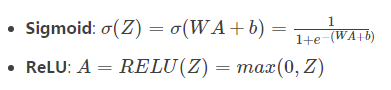
To implement LINEAR - > ACTIVATION, we use the following formula: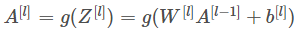Among them, function g will be sigmoid() or relu(), of course, sigmoid() is only used in the output layer. Now we formally construct the forward linear activation part.

For convenience, you will combine two functions (linear and activation) into one function (linear - > activation). Therefore, you will implement a function that first performs the linear forward step and then the activation forward step.

# GRADED FUNCTION: linear_activation_forward

def linear_activation_forward(A_prev, W, b, activation):
    """
    //Forward propagation of LINEAR - > ACTIVATION layer

    //Parameters:
        A_prev - Activation from the upper layer (or input layer), with dimensions of(Number of nodes in the previous layer, number of examples)
        W - Weight matrix, numpy Array, dimension is (number of nodes in the current layer, size of the previous layer)
        b - Partial vectors, numpy Array, dimension (number of nodes at current level, 1)
        activation - Select the activation function name, string type used in this layer.["sigmoid" | "relu"]

    //Return:
        A - The output of the activation function, also known as the activated value
        cache - A Containment“ linear_cache"And " activation_cache"For our dictionary, we need to store it to efficiently compute backward delivery
    """
    
    if activation == "sigmoid":
        # Inputs: "A_prev, W, b". Outputs: "A, activation_cache".
        ### START CODE HERE ### (≈ 2 lines of code)
        Z, linear_cache = linear_forward(A_prev, W, b)
        A, activation_cache = sigmoid(Z)
        ### END CODE HERE ###
    
    elif activation == "relu":
        # Inputs: "A_prev, W, b". Outputs: "A, activation_cache".
        ### START CODE HERE ### (≈ 2 lines of code)
        Z, linear_cache = linear_forward(A_prev, W, b)
        A, activation_cache = relu(Z)
        ### END CODE HERE ###
    
    assert (A.shape == (W.shape[0], A_prev.shape[1]))
    cache = (linear_cache, activation_cache)

    return A, cache

Test:

A_prev, W, b = linear_activation_forward_test_case()

A, linear_activation_cache = linear_activation_forward(A_prev, W, b, activation = "sigmoid")
print("With sigmoid: A = " + str(A))

A, linear_activation_cache = linear_activation_forward(A_prev, W, b, activation = "relu")
print("With ReLU: A = " + str(A))

Result:

With sigmoid: A = [[0.96890023 0.11013289]]
With ReLU: A = [[3.43896131 0.        ]]

Note: In deep learning, "[LINEAR-> ACTIVATION]" computation is regarded as a single layer rather than two layers in neural networks.

 

4.3-L Layer Model

To make it easier to implement L-layer neural networks, you will need a function that copies the previous function (linear_activation_forward with RELU) L times and then 1 time with a linear_activation_forward with SIGMOID.

Exercise: Realize the forward propagation of the above model.

Description: In the following code, AL represents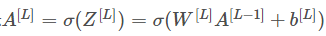(Also known as Yhat, mathematically expressed as Y ^.)
Tips:

• Use the functions you wrote earlier
• Reproduce [LINEAR - > RELU] (L-1) times using for loop
• Don't forget to track caches in the Cache list. To add a new value C to the list, use list.append(c)

# GRADED FUNCTION: L_model_forward

def L_model_forward(X, parameters):
    """
    //Realize [LINEAR - > RELU]* (L-1) - > LINEAR - > SIGMOID computing forward propagation, that is, forward propagation of multi-layer network, and perform LINEAR and ACVATION for each layer behind.

    //Parameters:
        X - Data, numpy Array, dimension (number of input nodes, number of examples)
        parameters - initialize_parameters_deep()Output of

    //Return:
        AL - Final activation value
        caches - A list of caches containing the following:
                 linear_relu_forward()Each cache(Yes L-1 Number, index from 0 to L-2)
                 linear_sigmoid_forward()Of cache(Only one, indexed as L-1)
    """

    caches = []
    A = X
    L = len(parameters) // 2                  # number of layers in the neural network
    print("keys in parameters: ", parameters.keys())
    # Implement [LINEAR -> RELU]*(L-1). Add "cache" to the "caches" list.
    for l in range(1, L):
        A_prev = A 
        ### START CODE HERE ### (≈ 2 lines of code)
        A, cache = linear_activation_forward(A_prev, parameters['W' + str(l)], parameters['b' + str(l)], "relu")
        caches.append(cache)

        ### END CODE HERE ###
    
    # Implement LINEAR -> SIGMOID. Add "cache" to the "caches" list.
    ### START CODE HERE ### (≈ 2 lines of code)
    AL, cache = linear_activation_forward(A, parameters['W' + str(L)], parameters['b' + str(L)], "sigmoid")
    caches.append(cache)

    ### END CODE HERE ###
    
    assert(AL.shape == (1,X.shape[1]))
            
    return AL, caches

Test:

X, parameters = L_model_forward_test_case()
AL, caches = L_model_forward(X, parameters)
print("AL = " + str(AL))
print("Length of caches list = " + str(len(caches)))

Result:

keys in parameters:  dict_keys(['W1', 'b1', 'W2', 'b2'])
AL = [[0.17007265 0.2524272 ]]
Length of caches list = 2

Great. Now you have a complete forward propagation that accepts input X and outputs a row vector A[L] containing your prediction. It also records all intermediate values in "caches". Using A[L], you can calculate your projected cost.

 

5-Cost function

Now you will achieve forward and reverse propagation. You need to calculate the cost, because you want to check whether your model is really learning.

Exercise: Use the following formula to calculate cross-entropy cost J:

# GRADED FUNCTION: compute_cost

def compute_cost(AL, Y):
    """
    //Implementing the cost function defined in Equation (4).

    //Parameters:
        AL - The probability vector corresponding to label prediction is dimension (1, number of examples)
        Y - Tag vectors (e.g., 0 if not cat, 1 if cat) and dimensions (1, number)

    //Return:
        cost - Cross Entropy Cost
    """
    
    m = Y.shape[1]

    # Compute loss from aL and y.
    ### START CODE HERE ### (≈ 1 lines of code)
#     cost = -np.sum(np.multiply(np.log(AL),Y) + np.multiply(np.log(1 - AL), 1 - Y)) / m
    cost = -np.sum((np.log(AL)*Y) + np.log(1 - AL)*(1 - Y)) / m
    ### END CODE HERE ###
    
    cost = np.squeeze(cost)      # To make sure your cost's shape is what we expect (e.g. this turns [[17]] into 17).
    assert(cost.shape == ())
    
    return cost

Test:

Y, AL = compute_cost_test_case()

print("cost = " + str(compute_cost(AL, Y)))

Result:

cost = 0.414931599615397

 

6 - Back Propagation Module

Just like forward propagation, you will implement help functions for back propagation. Keep in mind that back propagation is used to calculate the gradient of the loss function relative to the parameter. Reminder:

Now, like forward propagation, you will build back propagation in three steps:

• LINEAR backward
• LINEAR - > ACTIVATION backward where ACTIVATION activation calculates the derivatives of ReLU or sigmoid activation
• [LINEAR-> RELU] *L-1-> LINEAR-> SIGMOID backward (whole model)

 

 

6.1 - Linear Backward

For the linear part of the equation:

 

Exercise: Use the three formulas above to implement linear_backward().

# GRADED FUNCTION: linear_backward

def linear_backward(dZ, cache):
    """
    //The Linear Part of Back Propagation for Single Layer (Layer L)

    //Parameters:
         dZ - Relative to (current section) l Cost Gradient of Layer Linear Output
         cache - Tuples of values propagating forward from the current layer( A_prev，W，b)

    //Return:
         dA_prev - Relative to activation (front layer) l-1)Cost gradient, and A_prev Dimensions are the same
         dW - Be relative to W(Current Layer l)Cost gradient, and W The same dimension
         db - Be relative to b(Current Layer l)Cost gradient, and b Dimensions are the same
    """
    A_prev, W, b = cache
    m = A_prev.shape[1]
    
    ### START CODE HERE ### (≈ 3 lines of code)
    dW = np.dot(dZ, A_prev.T) / m
    db = np.sum(dZ, axis=1, keepdims=True) / m
    dA_prev = np.dot(W.T, dZ)
    ### END CODE HERE ###
    
    assert (dA_prev.shape == A_prev.shape)
    assert (dW.shape == W.shape)
    assert (db.shape == b.shape)
    
    return dA_prev, dW, db

Test:

# Set up some test inputs
dZ, linear_cache = linear_backward_test_case()

dA_prev, dW, db = linear_backward(dZ, linear_cache)
print ("dA_prev = "+ str(dA_prev))
print ("dW = " + str(dW))
print ("db = " + str(db))

Result:

dA_prev = [[ 0.51822968 -0.19517421]
 [-0.40506361  0.15255393]
 [ 2.37496825 -0.89445391]]
dW = [[-0.10076895  1.40685096  1.64992505]]
db = [[0.50629448]]

 

6.2-Linear-Reverse Activation

Next, you will create a function that combines two auxiliary functions: the linear reverse step and the activation of the linear reverse step. To help you achieve linear activation inversion, we provide two inversion functions:

• sigmoid_backward: The backpropagation of sigmoid () function is implemented. You can call it as follows:

dZ = sigmoid_backward(dA, activation_cache)

• relu_backward: This implements the reverse propagation of relu () function. You can call it as follows:

dZ = relu_backward(dA, activation_cache)

If g(.) is an activation function, sigmoid_backward and relu_backward are calculated as follows:

Exercise: Back propagation for LINEAR - > ACTIVATION layer.

# GRADED FUNCTION: linear_activation_backward

def linear_activation_backward(dA, cache, activation):
    """
    //Realize the backward propagation of LINEAR - > ACTIVATION layer.

    //Parameters:
         dA - Current Layer l Activated gradient
         cache - The tuple we store for validly calculating the value of backpropagation (the value is linear_cache，activation_cache)
         activation - The activation function name, string type to be used in this layer,["sigmoid" | "relu"]
    //Return:
         dA_prev - Relative to activation (front layer) l-1)Cost gradient value, and A_prev Dimensions are the same
         dW - Be relative to W(Current Layer l)Cost gradient value, and W The same dimension
         db - Be relative to b(Current Layer l)Cost gradient value, and b The same dimension
    """
    linear_cache, activation_cache = cache
    
    if activation == "relu":
        ### START CODE HERE ### (≈ 2 lines of code)
        dZ = relu_backward(dA, activation_cache)
        dA_prev, dW, db = linear_backward(dZ, linear_cache)
        ### END CODE HERE ###
        
    elif activation == "sigmoid":
        ### START CODE HERE ### (≈ 2 lines of code)
        dZ = sigmoid_backward(dA, activation_cache)
        dA_prev, dW, db = linear_backward(dZ, linear_cache)
        ### END CODE HERE ###
    
    return dA_prev, dW, db

Test:

AL, linear_activation_cache = linear_activation_backward_test_case()

dA_prev, dW, db = linear_activation_backward(AL, linear_activation_cache, activation = "sigmoid")
print ("sigmoid:")
print ("dA_prev = "+ str(dA_prev))
print ("dW = " + str(dW))
print ("db = " + str(db) + "\n")

dA_prev, dW, db = linear_activation_backward(AL, linear_activation_cache, activation = "relu")
print ("relu:")
print ("dA_prev = "+ str(dA_prev))
print ("dW = " + str(dW))
print ("db = " + str(db))

Result:

sigmoid:
dA_prev = [[ 0.11017994  0.01105339]
 [ 0.09466817  0.00949723]
 [-0.05743092 -0.00576154]]
dW = [[ 0.10266786  0.09778551 -0.01968084]]
db = [[-0.05729622]]

relu:
dA_prev = [[ 0.44090989  0.        ]
 [ 0.37883606  0.        ]
 [-0.2298228   0.        ]]
dW = [[ 0.44513824  0.37371418 -0.10478989]]
db = [[-0.20837892]]

 

6.3-L-backward model

Now you will implement backward functionality for the entire network. Recall that when you implement the L_model_forward function, you store a cache containing (X, W, b and z) in each iteration. In the reverse propagation module, you will use these variables to calculate the gradient. Therefore, in the L_model_backward function, you will traverse all hidden layers backwards from layer L. In each step, you will use the cache value of Layer L to traverse Layer L backwards. Figure 5 below shows a backward traversal.

In the previous forward calculation, we stored some caches containing (X, W, b and z), which we will use to calculate the gradient values in the ship that committed the crime. So in the L-layer model, we need to traverse all the hidden layers from the L-layer. In each step, we need to use the cache values of that layer to calculate the gradient values. Reverse propagation.  
Above we mentioned A[L], which belongs to the output layer, A[L] = _ (Z[L]), so we need to calculate dAL. We can use the following code to calculate it:

dAL = - (np.divide(Y, AL) - np.divide(1 - Y, 1 - AL)) # derivative of cost with respect to AL

Then, you can use this activated gradient dAL to continue moving backwards. As shown in Figure 5, you can now enter dAL into the LINEAR - > SIGMOID backward function that you implement (it will use the cached value stored by the L_model_forward function). After that, you must use the for loop and use the LINEAR - > RELU backward function to iterate over all other layers. You should store each dA, dW, and db in the gradient dictionary. To this end, use the following formula:

For example, for l=3, this stores dW[l] in the gradient ["dW 3"].

 

Exercise: Implement backpropagation for [LINEAR-> RELU] * (L-1) -> LINEAR-> SIGMOID model.

# GRADED FUNCTION: L_model_backward

def L_model_backward(AL, Y, caches):
    """
    //Back propagation of [LINEAR-> RELU]* (L-1) - > LINEAR - > SIGMOID group is the backward propagation of multi-layer networks.

    //Parameters:
     AL - Probability Vector, Output of Forward Propagation( L_model_forward())
     Y - Tag vectors (e.g., 0 if not cat, 1 if cat) and dimensions (1, number)
     caches - Containing the following cache List:
                 linear_activation_forward("relu")Of cache，No Output Layer
                 linear_activation_forward("sigmoid")Of cache

    //Return:
     grads - Dictionary with Gradient Value
              grads ["dA"+ str(l)] = ...
              grads ["dW"+ str(l)] = ...
              grads ["db"+ str(l)] = ...
    """
    grads = {}
    L = len(caches) # the number of layers
    m = AL.shape[1]
    Y = Y.reshape(AL.shape) # after this line, Y is the same shape as AL

    # Initializing the backpropagation
    ### START CODE HERE ### (1 line of code)
    dAL = - (np.divide(Y, AL) - np.divide(1 - Y, 1 - AL))
    ### END CODE HERE ###
    
    # Lth layer (SIGMOID -> LINEAR) gradients. Inputs: "AL, Y, caches". Outputs: "grads["dAL"], grads["dWL"], grads["dbL"]
    ### START CODE HERE ### (approx. 2 lines)
    current_cache = caches[L-1]
    grads["dA" + str(L)], grads["dW" + str(L)], grads["db" + str(L)] = linear_activation_backward(dAL, current_cache, "sigmoid")
    ### END CODE HERE ###
    
    for l in reversed(range(L - 1)):
        # lth layer: (RELU -> LINEAR) gradients.
        # Inputs: "grads["dA" + str(l + 2)], caches". Outputs: "grads["dA" + str(l + 1)] , grads["dW" + str(l + 1)] , grads["db" + str(l + 1)] 
        ### START CODE HERE ### (approx. 5 lines)
        current_cache = caches[l]
        grads["dA" + str(l + 1)] , grads["dW" + str(l + 1)] , grads["db" + str(l + 1)]  = linear_activation_backward(grads["dA" + str(l + 2)], current_cache, "relu")
        ### END CODE HERE ###

    return grads

Test:

AL, Y_assess, caches = L_model_backward_test_case()
grads = L_model_backward(AL, Y_assess, caches)
print ("dW1 = "+ str(grads["dW1"]))
print ("db1 = "+ str(grads["db1"]))
print ("dA1 = "+ str(grads["dA1"]))

Result:

dW1 = [[0.41010002 0.07807203 0.13798444 0.10502167]
 [0.         0.         0.         0.        ]
 [0.05283652 0.01005865 0.01777766 0.0135308 ]]
db1 = [[-0.22007063]
 [ 0.        ]
 [-0.02835349]]
dA1 = [[ 0.          0.52257901]
 [ 0.         -0.3269206 ]
 [ 0.         -0.32070404]
 [ 0.         -0.74079187]]

 

6.4 - Update parameters

In this section, you will update the model parameters using gradient descent:

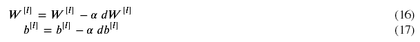
Among them, alpha is the learning rate. After calculating the updated parameters, they are stored in the parameter dictionary.

Exercise: Implement update_parameters() using gradient descent to update parameters.

Description: Use gradient descent to update parameter l=1, 2,..., L for each W[L] and b[L].

# GRADED FUNCTION: update_parameters

def update_parameters(parameters, grads, learning_rate):
    """
    //Updating parameters using gradient descent

    //Parameters:
     parameters - A dictionary containing your parameters
     grads - A dictionary containing gradient values is L_model_backward Output of

    //Return:
     parameters - Dictionary with update parameters
                   //The parameter ["W"+str(l)]=...
                   //The parameter ["b"+str(l)]=...
    """
    
    L = len(parameters) // 2 # number of layers in the neural network
    # Update rule for each parameter. Use a for loop.
    ### START CODE HERE ### (≈ 3 lines of code)
    for l in range(L):
        parameters["W" + str(l+1)] = parameters["W" + str(l + 1)] - learning_rate * grads["dW" + str(l + 1)]
        parameters["b" + str(l+1)] = parameters["b" + str(l + 1)] - learning_rate * grads["db" + str(l + 1)]
    ### END CODE HERE ###
        
    return parameters

Test:

parameters, grads = update_parameters_test_case()
parameters = update_parameters(parameters, grads, 0.1)

print ("W1 = "+ str(parameters["W1"]))
print ("b1 = "+ str(parameters["b1"]))
print ("W2 = "+ str(parameters["W2"]))
print ("b2 = "+ str(parameters["b2"]))

Result:

W1 = [[-0.59562069 -0.09991781 -2.14584584  1.82662008]
 [-1.76569676 -0.80627147  0.51115557 -1.18258802]
 [-1.0535704  -0.86128581  0.68284052  2.20374577]]
b1 = [[-0.04659241]
 [-1.28888275]
 [ 0.53405496]]
W2 = [[-0.55569196  0.0354055   1.32964895]]
b2 = [[-0.84610769]]

 

7 - Conclusion

Congratulations on all the functions you need to build a deep neural network! We know that this is a long task, but it will only get better in the future. The next part of the assignment is easier. In the next assignment, you will put all of this together to build two models:

• A Two-Layer Neural Network
• A L-Layer Neural Network

In fact, you will use these models to classify cat and non-cat images!