In this Lab, we will implement the basic function of gradient descent algorithm to find the data boundary in small data set First, we will start with some functions to help us draw and visualize data.

import matplotlib.pyplot as plt
import numpy as np
import pandas as pd

#Some helper functions for plotting and drawing lines

def plot_points(X, y):
    admitted = X[np.argwhere(y==1)]
    rejected = X[np.argwhere(y==0)]
    plt.scatter([s[0][0] for s in rejected], [s[0][1] for s in rejected], s = 25, color = 'blue', edgecolor = 'k')
    plt.scatter([s[0][0] for s in admitted], [s[0][1] for s in admitted], s = 25, color = 'red', edgecolor = 'k')

def display(m, b, color='g--'):
    plt.xlim(-0.05,1.05)
    plt.ylim(-0.05,1.05)
    x = np.arange(-10, 10, 0.1)
    plt.plot(x, m*x+b, color)

Reading and drawing data

data = pd.read_csv('data.csv', header=None)
X = np.array(data[[0,1]])
y = np.array(data[2])
plot_points(X,y)
plt.show()

Implement basic functions

# Implement the following functions

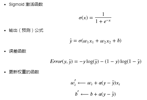
# Activation (sigmoid) function
def sigmoid(x):
    return 1 / (1 + np.exp(-x))

# Output (prediction) formula
def output_formula(features, weights, bias):
    return sigmoid(np.dot(features, weights) + bias)

# Error (log-loss) formula
def error_formula(y, output):
    return - y*np.log(output) - (1 - y) * np.log(1-output)

# Gradient descent step
def update_weights(x, y, weights, bias, learnrate):
    output = output_formula(x, weights, bias)
    d_error = -(y - output)
    weights -= learnrate * d_error * x
    bias -= learnrate * d_error
    return weights, bias

Training function

This function will help us to iterate the gradient descent algorithm through all the data for multiple epoch s It will also draw data and some boundary lines as we run the algorithm.

np.random.seed(44)

epochs = 100
learnrate = 0.01

def train(features, targets, epochs, learnrate, graph_lines=False):
    
    errors = []
    n_records, n_features = features.shape
    last_loss = None
    weights = np.random.normal(scale=1 / n_features**.5, size=n_features)
    bias = 0
    for e in range(epochs):
        del_w = np.zeros(weights.shape)
        for x, y in zip(features, targets):
            output = output_formula(x, weights, bias)
            error = error_formula(y, output)
            weights, bias = update_weights(x, y, weights, bias, learnrate)
        
        # Printing out the log-loss error on the training set
        out = output_formula(features, weights, bias)
        loss = np.mean(error_formula(targets, out))
        errors.append(loss)
        if e % (epochs / 10) == 0:
            print("\n========== Epoch", e,"==========")
            if last_loss and last_loss < loss:
                print("Train loss: ", loss, "  WARNING - Loss Increasing")
            else:
                print("Train loss: ", loss)
            last_loss = loss
            predictions = out > 0.5
            accuracy = np.mean(predictions == targets)
            print("Accuracy: ", accuracy)
        if graph_lines and e % (epochs / 100) == 0:
            display(-weights[0]/weights[1], -bias/weights[1])
            

    # Plotting the solution boundary
    plt.title("Solution boundary")
    display(-weights[0]/weights[1], -bias/weights[1], 'black')

    # Plotting the data
    plot_points(features, targets)
    plt.show()

    # Plotting the error
    plt.title("Error Plot")
    plt.xlabel('Number of epochs')
    plt.ylabel('Error')
    plt.plot(errors)
    plt.show()