statement

Reference in this article He Guang

Preface

Structure of this paper:
First, a complete convolutional neural network module is built from the bottom layer, and then it is implemented by tensorflow.

The model structure is as follows: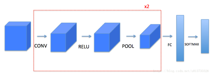

Function function of the module to be implemented:

• Convolution module, including the following functions:
  • Expand boundary with 0
  • Convolution window
  • Forward convolution
  • Inverse convolution
• The pooling module contains the following functions:
  • Forward pooling
  • Create mask
  • Value assignment
  • Reverse pool

1, Convolutional neural network

1.1 import library

import numpy as np
import h5py
import matplotlib.pyplot as plt

plt.rcParams['figure.figsize'] = (5.0,4.0)
plt.rcParams['image.interpolation'] = 'nearest'
plt.rcParams['image.cmap'] = 'gray'

np.random.seed(1)

1.2 boundary filling

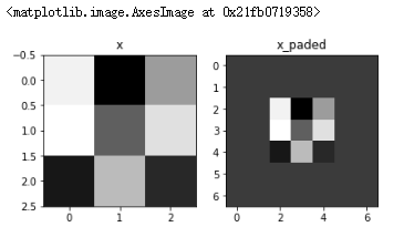
NP pad is used for boundary filling.

def zero_pad(X,pad):
    """
    Use 0 to e x pand the width and height of pad.
    
    Parameters:
        X - image data set, dimension is (number of samples, image height, image width, number of image channels)
        pad - integer, the amount of padding per image in the vertical and horizontal dimensions
    Return:
        X_pasted - the expanded image data set. The dimension is (number of samples, image height + 2*pad, image width + 2*pad, number of image channels)
    """
    X_paded = np.pad(X,((0,0),(pad,pad),(pad,pad),(0,0)),'constant')
    return X_paded

Test:

np.random.seed(1)
x = np.random.randn(4,3,3,2)
x_paded = zero_pad(x,2)

print(x.shape,x_paded.shape,x[1,1],x_paded[1,1])

fig,axarr = plt.subplots(1,2)
axarr[0].set_title('x')
axarr[0].imshow(x[0,:,:,0])
axarr[1].set_title('x_paded')
axarr[1].imshow(x_paded[0,:,:,0])

Result:

(4, 3, 3, 2) (4, 7, 7, 2) [[ 0.90085595 -0.68372786]
 [-0.12289023 -0.93576943]
 [-0.26788808  0.53035547]] [[0. 0.]
 [0. 0.]
 [0. 0.]
 [0. 0.]
 [0. 0.]
 [0. 0.]
 [0. 0.]]

1.3 single step convolution

Filter size f=3, step s=1, fill pad=2.

def conv_single_step(a_slice_prev,W,b):
   """
   Apply a filter defined by the parameter W to a fragment of the active output of the previous layer. Here the slice size is the same as the filter size.
   
   Parameters:
       A ﹣ slice ﹣ prev - a piece of input data with dimensions (filter size, filter size, number of previous channels)
       W - weight parameter, included in a matrix, dimension is (filter size, filter size, number of previous channels)
       b - offset parameter, contained in a matrix with dimensions (1,1,1)
   Return:
       Z - the result of convoluting the sliding window (W,b) on the slice x of the input data.
   """
   s = a_slice_prev*W+b
   Z = np.sum(s)
   return Z

Test:

np.random.seed(1)
a_slice_prev = np.random.randn(4,4,3)
W = np.random.randn(4,4,3)
b = np.random.randn(1,1,1)

Z = conv_single_step(a_slice_prev,W,b)
print(Z)

Result:

-23.16021220252078

1.4 forward propagation of convolution layer

def conv_forward(A_prev,W,b,hparameters):
   """
   //Forward propagation of convolution function
   
   //Parameters:
       A_prev - The activation output matrix of the upper layer, dimension is( m，n_H_prev,n_C_prev),(Number of samples, height of previous image, width of previous image, number of previous filters)
       W - Weight matrix, dimension is( f，f,n_C_prev,n_c),(Filter size, filter size, number of filters in the previous layer, number of filters in this layer)
       b - Offset matrix with dimensions (1, 1, 1, n_C)，(1，1，1，Number of filters on this floor)
       hparameters - Contains " stride"And " pad"The super parameter dictionary for.
   //Return:
       Z - Convolution output, dimension is( m,n_H,n_W,n_C),(Number of samples, height of image, broadband of image, number of filters)
       cache - Some back propagation functions are cached conv_backward()Some data needed
   """
   (m,n_H_prev,n_W_rev,n_C_prev) = A_prev.shape
   (f,f,n_C_prev,n_C) = W.shape
   stride = hparameters['stride']
   pad = hparameters['pad']
   n_H = int((n_H_prev+2*pad-f)/stride)+1
   n_W = int((n_W_rev+2*pad-f)/stride)+1
   
   Z = np.zeros((m,n_H,n_W,n_C))
   A_prev_pad = zero_pad(A_prev,pad)
   
   for i in range(m):
       a_prev_pad = A_prev_pad[i]
       for h in range(n_H):
           for w in range(n_W):
               for c in range(n_C):
                   vert_start = h*stride
                   vert_end = vert_start+f
                   horiz_start = w*stride
                   horiz_end = horiz_start+f
                   a_slip_prev = a_prev_pad[vert_start:vert_end,horiz_start:horiz_end,:]
                   Z[i,h,w,c] = conv_single_step(a_slip_prev,W[:,:,:,c],b[0,0,0,c])
   
   cache = (A_prev,W,b,hparameters)
   return (Z,cache)

Test:

np.random.seed(1)

A_prev = np.random.randn(10,4,4,3)
W = np.random.randn(2,2,3,8)
b = np.random.randn(1,1,1,8)

hparameters = {'pad':2,'stride':1}

Z,cache_conv = conv_forward(A_prev,W,b,hparameters)

print(np.mean(Z))
print(cache_conv[0][1][2][3])

Result:

0.15585932488906465
[-0.20075807  0.18656139  0.41005165]

1.5 forward propagation of pool layer

def pool_forward(A_prev,hparameters,mode='max'):
   """
   //Forward propagation of pooling layer
   
   //Parameters:
       A_prev - Input data, dimension is( m,n_H_prev,n_W_prev,n_C_prev)
       hparameters - Contains'f'and'stride'Super parameter Dictionary of
       mode - Mode selection['max'|'average']
   //Return:
       A - Output of pooling layer, dimension is( m,n_H,n_W,n_C)
       cache - Some back propagation values are stored, including the dictionary of input and super parameters.
   """
   (m,n_H_prev,n_W_prev,n_C_prev)=A_prev.shape
   f = hparameters['f']
   stride = hparameters['stride']
   n_H = int((n_H_prev-f)/stride)+1
   n_W = int((n_W_prev-f)/stride)+1
   n_C = n_C_prev
   A = np.zeros((m,n_H,n_W,n_C))
   
   for i in range(m):
       a_prev = A_prev[i]
       for h in range(n_H):
           for w in range(n_W):
               for c in range(n_C):
                   vert_start = h*stride
                   vert_end = vert_start+f
                   horiz_start = w*stride
                   horiz_end = horiz_start+f
                   a_slice_prev = a_prev[vert_start:vert_end,horiz_start:horiz_end,c]
                   
                   if mode=='max':
                       A[i,h,w,c] = np.max(a_slice_prev)
                   elif mode=='average':
                       A[i,h,w,c] = np.mean(a_slice_prev)
   cache = (A_prev,hparameters)
   return A,cache

Test:

np.random.seed(1)

A_prev = np.random.randn(2,4,4,3)

hparameters = {'f':4,'stride':1}

A,cache = pool_forward(A_prev,hparameters,mode='max')
print(A)
A,cache = pool_forward(A_prev,hparameters,mode='average')
print(A)

Result:

[[[[1.74481176 1.6924546  2.10025514]]]


 [[[1.19891788 1.51981682 2.18557541]]]]
[[[[-0.09498456  0.11180064 -0.14263511]]]


 [[[-0.09525108  0.28325018  0.33035185]]]]

1.6 back propagation of convolution layer

1.6.1 calculation of dA

dA+=∑h=0nH∑w=0nWWC×dZhwdA+=\sum_{h=0}^{n_H} \sum_{w=0}^{n_W} W_C \times dZ_{hw}dA+=h=0∑nH​​w=0∑nW​​WC​×dZhw​
Where, WCW ﹣ CWC is the filter, zhwz ﹣ hwzh w is a scalar, and zhwz ﹣ hwzh w is the gradient of output Z calculated by point multiplication of the h row and w column of the convolution layer. It should be noted that each time dA is updated, the same filter WCW ﹣ CWC will be multiplied by different dZ. Because in the forward propagation, each filter and a ﹣ slice are point multiplied and added. Therefore, when dA is calculated, the gradient of a ﹣ slice needs to be added. You can add a code in the loop:

da_perv_pad[vert_start:vert_end,horiz_start:horiz_end,:] += W[:,:,:,c] * dZ[i,h,w,c]

1.6.2 calculation of dW

dWc+=∑h=0nH∑w=0nWaslice×dZhwdW_c+=\sum_{h=0}^{n_H} \sum_{w=0}^{n_W} a_{slice} \times dZ_{hw}dWc​+=h=0∑nH​​w=0∑nW​​aslice​×dZhw​
Among them, aslicea {slice} aslice corresponds to the activation value of zijz {ij} Zij. Therefore, the gradient of W can be deduced. Because the filter is used to slide the data window, in fact, slices of the same size as the filter are cut out here, and as many times as they are cut, there are as many gradients. Therefore, they need to be added together to get the overall dW of this dataset.

dW[:,:,:, c] += a_slice * dZ[i , h , w , c]

1.6.2 calculation db

db+=∑h=0nH∑w=0nWdZhwdb+=\sum_{h=0}^{n_H} \sum_{w=0}^{n_W} dZ_{hw}db+=h=0∑nH​​w=0∑nW​​dZhw​

db[:,:,:,c] += dZ[ i, h, w, c]

def conv_backward(dZ,cache):
   """
   //Realizing the back propagation of the volume layer
   
   //Parameters:
       dZ - Output of convolution layer z The dimension is( m,n_H,n_W,n_C)
       cache - Parameters required for back propagation, conv_forward()One of the outputs of
   //Return:
       dA_prev - Input of convolution layer(A_prev)The gradient value of, dimension is( m,n_H_prev,n_W_prev,n_C_prev)
       dW - The gradient of the weight of the convolution layer, dimension is( f,f,n_C_prev,n_C)
       db - The gradient of the bias of the convolution layer is (1, 1, 1, n_C)
   """
   (A_prev,W,b,hparameters) = cache

   (m,n_H_prev,n_W_prev,n_C_prev) = A_prev.shape
   
   (m,n_H,n_W,n_C) = dZ.shape
   
   (f,f,n_C_prev,n_C) = W.shape
   
   pad = hparameters['pad']
   stride = hparameters['stride']
   
   dA_prev = np.zeros((m,n_H_prev,n_W_prev,n_C_prev))
   dW = np.zeros((f,f,n_C_prev,n_C))
   db = np.zeros((1,1,1,n_C))
   
   A_prev_pad = zero_pad(A_prev,pad)
   dA_prev_pad = zero_pad(dA_prev,pad)
   
   for i in range(m):
       a_prev_pad = A_prev_pad[i]
       da_prev_pad = dA_prev_pad[i]
       
       for h in range(n_H):
           for w in range(n_W):
               for c in range(n_C):
                   vert_start = h
                   vert_end = vert_start+f
                   horiz_start = w
                   horiz_end = horiz_start+f
                   
                   a_slice = a_prev_pad[vert_start:vert_end,horiz_start:horiz_end,:]
                   da_prev_pad[vert_start:vert_end,horiz_start:horiz_end,:]+=W[:,:,:,c]*dZ[i,h,w,c]
                   dW[:,:,:,c] += a_slice*dZ[i,h,w,c]
                   db[:,:,:,c] += dZ[i,h,w,c]
       dA_prev[i,:,:,:] = da_prev_pad[pad:-pad,pad:-pad,:]
   assert(dA_prev.shape==(m,n_H_prev,n_W_prev,n_C_prev))
   
   return dA_prev,dW,db

Test:

np.random.seed(1)

A_prev = np.random.randn(10,4,4,3)
W = np.random.randn(2,2,3,8)
b = np.random.randn(1,1,1,8)
hparameters = {'pad':2,'stride':1}

Z,cache_conv = conv_forward(A_prev,W,b,hparameters)
dA_prev,dW,db = conv_backward(Z,cache_conv)

print(np.mean(dA_prev),np.mean(dW),np.mean(db))

Result:

9.608990675868995 10.581741275547566 76.37106919563735

1.7. Back propagation of pooling layer

1.7.1 back propagation of maximum pooling layer

First of all, we need to create a function to create "Mask" from "window(). This function creates a mask matrix to save the location of the maximum value. When it is 1, it represents the location of the maximum value. The others are 0. This is the maximum pooling layer.
Why create this mask matrix? Because we need to record the location of the maximum value so that it can be propagated back to the volume layer.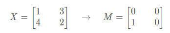

def create_mask_from_window(x):
   """
   Creates a mask from the input matrix to hold the location of the maximum matrix.
   
   Parameters:
       x - a matrix with dimension (F, f)
   Return:
       mask - matrix containing the position of the maximum value of x
   """
   mask = x == np.max(x)
   
   return mask

Test:

np.random.seed(1)

x = np.random.randn(2,3)
mask = create_mask_from_window(x)
print(x,mask)

Result:

[[ 1.62434536 -0.61175641 -0.52817175]
 [-1.07296862  0.86540763 -2.3015387 ]] [[ True False False]
 [False False False]]

1.7.2 back propagation of mean pooling layer

Different from the maximum pooling layer, the mean pooling layer takes the mean value of the filter.

def distribute_value(dz,shape):
   """
   Given a value, it is evenly distributed to each matrix position according to the matrix size.
   Parameters:
       dz - real number of input
       shape - tuple, two values, n ﹣ h, n ﹣ w
   Return:
       A - a matrix with assigned values, all of which are the same.
   """
   (n_H,n_W) = shape
   
   average = dz/(n_H*n_W)
   
   a = np.ones(shape)*average
   
   return a

Test:

dz = 2
shape = (2,2)

a = distribute_value(dz,shape)
print(a)

Result:

[[0.5 0.5]
 [0.5 0.5]]

1.7.3 pool layer back propagation

def pool_backward(dA,cache,mode="max"):
   """
   //Realize the back propagation of pooling layer
   
   //Parameters:
       dA - The output gradient of the pooling layer is the same as the output dimension of the pooling layer
       cache - Parameters stored in forward propagation of pooling layer
       mode - Mode selection['max'|'average']
   //Return:
       dA_prev - The input gradient of the pool layer, and A_prev Same dimension for
   """
   (A_prev,hparameters) = cache
   f = hparameters['f']
   stride = hparameters['stride']
   
   (m,n_H_prev,n_W_prev,n_C_prev) = A_prev.shape
   (m,n_H,n_W,n_C) = dA.shape
   
   dA_prev = np.zeros_like(A_prev)
   
   for i in range(m):
       a_prev = A_prev[i]
       for h in range(n_H):
           for w in range(n_W):
               for c in range(n_C):
                   vert_start = h
                   vert_end = vert_start + f
                   horiz_start = w
                   horiz_end = horiz_start + f
                   
                   if mode == 'max':
                       a_prev_slice = a_prev[vert_start:vert_end,horiz_start:horiz_end,c]
                       mask = create_mask_from_window(a_prev_slice)
                       dA_prev[i,vert_start:vert_end,horiz_start:horiz_end,c]+=np.multiply(mask,dA[i,h,w,c])
                   elif mode == 'average':
                       da = dA[i,h,w,c]
                       shape = (f,f)
                       dA_prev[i,vert_start:vert_end,horiz_start:horiz_end,c]+=distribute_value(da,shape)
   assert(dA_prev.shape == A_prev.shape)
   
   return dA_prev

Test:

np.random.seed(1)

A_prev = np.random.randn(5,5,3,2)
W = np.random.randn(2,2,3,8)
b = np.random.randn(1,1,1,8)
hparameters = {'f':2,'stride':1}
A,cache = pool_forward(A_prev,hparameters)
dA = np.random.randn(5,4,2,2)

dA_prev = pool_backward(dA,cache,mode='max')
print(np.mean(dA),dA_prev[1,1])

dA_prev = pool_backward(dA,cache,mode='average')
print(np.mean(dA),dA_prev[1,1])

Result:

0.14026942447888846 [[ 0.          0.        ]
 [-0.72334716  2.42826793]
 [ 0.          0.        ]]
0.14026942447888846 [[-0.0103192   0.16889297]
 [-0.18083679  0.69818344]
 [-0.17051759  0.52929047]]

2, Convolutional neural network based on tensorflow

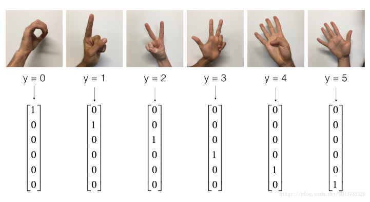
situation: use tensorflow to realize convolutional neural network, and then apply it to gesture recognition.

2.0 import library

import math
import numpy as np
import h5py
import matplotlib.pyplot as plt
import matplotlib.image as mpimg
import tensorflow as tf
from tensorflow.python.framework import ops

import cnn_utils
import tf_utils

np.random.seed(1)

Look inside:

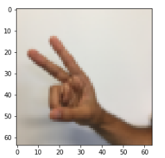
X_train_orig , Y_train_orig , X_test_orig , Y_test_orig , classes = tf_utils.load_dataset()
index = 6
plt.imshow(X_train_orig[index])
print(str(np.squeeze(Y_train_orig[:,index])))

Result:

2

Adjust the data to see the dimensions of the data:

X_train = X_train_orig/255
X_test = X_test_orig/255
Y_train = cnn_utils.convert_to_one_hot(Y_train_orig,6).T
Y_test = cnn_utils.convert_to_one_hot(Y_test_orig,6).T

print(X_train.shape[0],X_test.shape[0],X_train.shape,Y_train.shape,X_test.shape,Y_test.shape)

Result:

1080 120 (1080, 64, 64, 3) (1080, 6) (120, 64, 64, 3) (120, 6)

2.1. Create placeholders

tensorflow requires that placeholders be created for the input data that will be input into the model at session time. Because we use small batch data blocks, and the number of samples we input may not be fixed, we need to use None as the variable number in the number. The dimension of input X is [None, n ﹐ H0, n ﹐ W0, n ﹐ C0], and the corresponding Y is [None, n ﹐ Y].

def create_placeholders(n_H0,n_W0,n_C0,n_y):
   """
   Create placeholders for session s
   
   Parameters:
       N? H0 - real number, enter the height of the image
       N? W0 - real number, enter the width of the image
       N C0 - real number, number of channels entered
       n_y - real number, classified number
   Return:
       X - a placeholder for the input data. The dimension is [none, n [H0, n [W0, n [C0], and the type is' float '
       Y - placeholder for the label of the input data. The dimension is [none, n [y], and the type is' float '
   """
   X = tf.placeholder(tf.float32,[None,n_H0,n_W0,n_C0])
   Y = tf.placeholder(tf.float32,[None,n_y])
   return X,Y

Test:

X,Y = create_placeholders(64,64,3,6)
print(X,Y)

Result:

Tensor("Placeholder:0", shape=(?, 64, 64, 3), dtype=float32) Tensor("Placeholder_1:0", shape=(?, 6), dtype=float32)

2.2 initialization parameters

def initialize_parameters():
   """
   //Initialize the weight matrix. Here we hard code the weight matrix
   W1:[4,4,3,8]
   W2:[2,2,8,16]
   
   //Return:
       //Dictionary containing W1 and W2 of sensor type
   """
   tf.set_random_seed(1)
   
   W1 = tf.get_variable('W1',[4,4,3,8],initializer=tf.contrib.layers.xavier_initializer(seed=0))
   W2 = tf.get_variable('W2',[2,2,8,16],initializer=tf.contrib.layers.xavier_initializer(seed=0))
   
   parameters = {'W1':W1,'W2':W2}
   
   return parameters

Test:

tf.reset_default_graph()
with tf.Session() as sess_test:
    parameters = initialize_parameters()
    init = tf.global_variables_initializer()
    sess_test.run(init)
    print(parameters['W1'].eval()[1,1,1])
    print(parameters['W2'].eval()[1,1,1])
    
    sess_test.close()

Result:

[ 0.00131723  0.1417614  -0.04434952  0.09197326  0.14984085 -0.03514394
 -0.06847463  0.05245192]
[-0.08566415  0.17750949  0.11974221  0.16773748 -0.0830943  -0.08058
 -0.00577033 -0.14643836  0.24162132 -0.05857408 -0.19055021  0.1345228
 -0.22779644 -0.1601823  -0.16117483 -0.10286498]

2.3 forward propagation

Structure of the model:
conv2d->relu->maxpool->conv2d->relu->maxpool->fullconnected
Steps and parameters:

• Conv2d: step: 1, filling mode: 'SAME'
• Relu
• Max pool: filter size: 8x8, step: 8x8, fill mode: 'SAME'
• Conv2d: step: 1, filling mode: 'SAME'
• Relu
• Max pool: filter size: 4x4, step: 4x4, filling method: 'SAME'
• Output of one dimension upper layer
• Full connection layer (FC): use full connection layer without nonlinear activation function. There is no need to call softmax, which will result in six neurons in the output layer, which will then be passed to softmax.

def forward_propagation(X,parameters):
   """
   //Achieve forward propagation:
   conv2d->relu->maxpool->conv2d->relu->maxpool->flatten->fullyconnected
   
   //Parameters:
       X - Of input data placeholder，Dimension is (input node quantity, sample quantity)
       parameters - Contains'W1'and'W2'Of python Dictionaries
   //Return:
       Z3 - The last one linear Output of node
   """
   W1 = parameters['W1']
   W2 = parameters['W2']
   
   # Conv2d: step: 1, filling mode: 'SAME'
   Z1 = tf.nn.conv2d(X,W1,strides=[1,1,1,1],padding='SAME')
   # Relu
   A1 = tf.nn.relu(Z1)
   # Max pool: window size: 8x8, step: 8x8, fill mode: 'SAME'
   P1 = tf.nn.max_pool(A1,ksize=[1,8,8,1],strides=[1,8,8,1],padding='SAME')
   
   # Conv2d: step: 1, filling mode: 'SAME'
   Z2 = tf.nn.conv2d(P1,W2,strides=[1,1,1,1],padding='SAME')
   # Relu
   A2 = tf.nn.relu(Z2)
   # Max pool: window size: 4x4, step: 4x4, fill mode: 'SAME'
   P2 = tf.nn.max_pool(A2,ksize=[1,4,4,1],strides=[1,4,4,1],padding='SAME')
   
   # Output of one dimension upper layer
   P = tf.contrib.layers.flatten(P2)
   
   # Full connection layer (FC): use full connection layer without nonlinear activation function
   Z3 = tf.contrib.layers.fully_connected(P,6,activation_fn = None)
   
   return Z3

Test:

tf.reset_default_graph()
np.random.seed(1)

with tf.Session() as sess_test:
    X,Y = create_placeholders(64,64,3,6)
    parameters = initialize_parameters()
    Z3 = forward_propagation(X,parameters)
    init = tf.global_variables_initializer()
    sess_test.run(init)
    a = sess_test.run(Z3,{X:np.random.randn(2,64,64,3),Y:np.random.randn(2,6)})
    print(a)
    sess_test.close()

Result:

[[-0.44670227 -1.5720876  -1.5304923  -2.3101304  -1.2910438   0.46852064]
 [-0.17601591 -1.5797201  -1.4737016  -2.616721   -1.0081065   0.5747785 ]]

2.4 cost calculation

def compute_cost(Z3,Y):
   """
   Computational cost
   
   Parameters:
       Z3 - forward propagation of the output of the last linear node, dimension (6, number of samples)
       Y - placeholder of label vector, same dimension as Z3
   Return:
       Cost - calculated cost
   """
   cost = tf.reduce_mean(tf.nn.softmax_cross_entropy_with_logits(logits=Z3,labels=Y))
   return cost

Test:

tf.reset_default_graph()
with tf.Session() as sess_test:
    np.random.seed(1)
    X,Y = create_placeholders(64,64,3,6)
    parameters = initialize_parameters()
    Z3 = forward_propagation(X,parameters)
    cost = compute_cost(Z3,Y)
    
    init = tf.global_variables_initializer()
    sess_test.run(init)
    a = sess_test.run(cost,{X:np.random.randn(4,64,64,3),Y:np.random.randn(4,6)})
    print(a)
    sess_test.close()

Result:

2.9103398

2.5 building model

Steps:

• Create placeholder
• Initialization parameters
• Forward propagation
• Computational cost
• Back propagation
• Create optimizer
  Finally, you create a session to run the model.

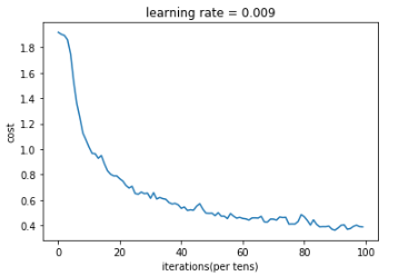
def model(X_train,Y_train,X_test,Y_test,learning_rate=0.009,num_epochs=100,minibatch_size=64,print_cost=True,isPlot=True):
   """
   //Using tensorflow to realize three-layer convolutional neural network
   conv2d->relu->maxpool->conv2d->relu->maxpool->flatten->fullyconnected
   
   //Parameters:
       X_train - Training data, dimension is(None, 64, 64, 3)
       Y_train - Label corresponding to training data, dimension is(None, n_y = 6)
       X_test - Test data, dimension is(None, 64, 64, 3)
       Y_test - Label corresponding to training data, dimension is(None, n_y = 6)
       learning_rate - Learning rate
       num_epochs - Number of traversals of the entire dataset
       minibatch_size - Size of each small batch of data block
       print_cost - Print cost value or not, print the entire dataset once every 100 iterations
       isPlot - Map or not
   //Return:
       train_accuracy - Real number, accuracy of training set
       test_accuracy - Real number, test set accuracy
       parameters - Parameters after learning
   """
   ops.reset_default_graph()
   tf.set_random_seed(1)
   seed = 3
   (m,n_H0,n_W0,n_C0) = X_train.shape
   n_y = Y_train.shape[1]
   costs = []
   X,Y = create_placeholders(n_H0,n_W0,n_C0,n_y)
   parameters = initialize_parameters()
   Z3 = forward_propagation(X,parameters)
   cost = compute_cost(Z3,Y)
   optimizer = tf.train.AdamOptimizer(learning_rate=learning_rate).minimize(cost)
   init = tf.global_variables_initializer()
   with tf.Session() as sess:
       sess.run(init)
       for epoch in range(num_epochs):
           minibatch_cost = 0
           num_minibatches = int(m/minibatch_size)
           seed = seed + 1
           minibatches = cnn_utils.random_mini_batches(X_train,Y_train,minibatch_size,seed)
           
           for minibatch in minibatches:
               (minibatch_X,minibatch_Y) = minibatch
               _,temp_cost = sess.run([optimizer,cost],feed_dict={X:minibatch_X,Y:minibatch_Y})
               minibatch_cost +=temp_cost/num_minibatches
           
           if print_cost:
               if epoch%5==0:
                   print('epoch=',epoch,',minibatch_cost=',minibatch_cost)
                   
           if epoch%1==0:
               costs.append(minibatch_cost)
       
       if isPlot:
           plt.plot(np.squeeze(costs))
           plt.ylabel('cost')
           plt.xlabel('iterations(per tens)')
           plt.title('learning rate = '+str(learning_rate))
           plt.show()
       
       predict_op = tf.arg_max(Z3,1)
       corrent_prediction = tf.equal(predict_op,tf.arg_max(Y,1))
       
       accuracy = tf.reduce_mean(tf.cast(corrent_prediction,'float'))
       print(accuracy)
       
       train_accurary = accuracy.eval({X:X_train,Y:Y_train})
       test_accuary = accuracy.eval({X:X_test,Y:Y_test})
       
       print(train_accurary)
       print(test_accuary)
       
       return (train_accurary,test_accuary,parameters)

Test:

_,_,parameters = model(X_train,Y_train,X_test,Y_test,num_epochs=100)

Result:

epoch= 0 ,minibatch_cost= 1.9179195687174797
epoch= 5 ,minibatch_cost= 1.5324752107262611
epoch= 10 ,minibatch_cost= 1.0148038603365421
epoch= 15 ,minibatch_cost= 0.8851366713643074
epoch= 20 ,minibatch_cost= 0.7669634483754635
epoch= 25 ,minibatch_cost= 0.651207884773612
epoch= 30 ,minibatch_cost= 0.6133557204157114
epoch= 35 ,minibatch_cost= 0.6059311926364899
epoch= 40 ,minibatch_cost= 0.5347129087895155
epoch= 45 ,minibatch_cost= 0.5514022018760443
epoch= 50 ,minibatch_cost= 0.49697646126151085
epoch= 55 ,minibatch_cost= 0.4544383566826582
epoch= 60 ,minibatch_cost= 0.45549566112458706
epoch= 65 ,minibatch_cost= 0.4583591800183058
epoch= 70 ,minibatch_cost= 0.4500396177172661
epoch= 75 ,minibatch_cost= 0.4106866829097271
epoch= 80 ,minibatch_cost= 0.46900513023138046
epoch= 85 ,minibatch_cost= 0.389252956956625
epoch= 90 ,minibatch_cost= 0.3638075301423669
epoch= 95 ,minibatch_cost= 0.3761322880163789
Tensor("Mean_1:0", shape=(), dtype=float32)
0.86851853
0.73333335