The data set we use is the movie review data set imdb provided by testnflow2

When loading data sets for the first time, it may be necessary to download data from the Internet, which is relatively slow. I put it on the network disk, and the download link is https://pan.baidu.com/s/1tq kw3tldmwn-cmtcbrplw
Extraction code: 4r7f

Copy it to after downloading

data = keras.datasets.imdb
#Limit the number of words read
max_word = 10000
(x_train, y_train), (x_test, y_test) = data.load_data(num_words=max_word)

View data shape

x_train.shape, y_train.shape

Output: ((25000,), (25000,))

View tab

print(y_train)
print(y_train.max())
print(y_train.min())

Output:

[1 0 0 ... 0 1 0]

1

0

Well, it's a dichotomy.

The length of input data of neural network should be the same. Let's see the length of training data

data_lens = [len(x) for x in x_train]
print(max(data_lens))
print(min(data_lens))

Output:

2494

11

Different length, our next step is to make it the same length, and the text is trained into a dense vector. If you don't understand, please query the relevant information by yourself, and don't introduce the theory much. This paper focuses on the implementation process. Let's look at the length distribution of the data

import matplotlib.pyplot as plt
import numpy as np
p_x = np.linspace(0,2494,len(data_lens))
p_y = data_lens
plt.scatter(p_x,p_y)

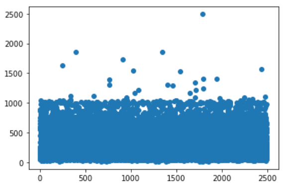
We fixed the length to a value greater than the average length, which is

np.mean(data_lens)

Output: 238.71364

OK, let's take 300

x_train = keras.preprocessing.sequence.pad_sequences(x_train,300)
x_test = keras.preprocessing.sequence.pad_sequences(x_test,300)

Start the model building, and the text intensive is completed by the functions in tensorflow2 model

model = keras.models.Sequential()
#Training text into dense vector, data dimension (max'word, 300) - > (max'word, 300, 50)
model.add(layers.Embedding(max_word,50,input_length=300))
#Add a flattening layer to flatten the data. The data dimension (max_word, 300,50) - > (max_word, 300 * 50) is convenient to transfer to the full connection layer
model.add(layers.Flatten())
#Add full connection layer
model.add(layers.Dense(128,activation='relu'))
#Add output layer
model.add(layers.Dense(1))
#sigmoid selection of activation function for binary classification problem
model.add(layers.Activation('sigmoid'))
#View built models
model.summary()

Output:

Start model compilation and training

model.compile(optimizer = keras.optimizers.Adam(lr=0.001) #Set optimizer and learning rate lr
              ,loss = 'binary_crossentropy' #Loss function binary cross entropy]
              ,metrics = ['acc']  #Accuracy of evaluation index acc
)
model.fit(x_train
          ,y_train
          ,epochs=10 #Training times
          ,batch_size = 128
          ,validation_data = (x_test,y_test)
         )

Train on 25000 samples, validate on 25000 samples Epoch 1/10 25000/25000 [==============================] - 7s 278us/sample - loss: 0.4376 - acc: 0.7748 - val_loss: 0.2951 - val_acc: 0.8735

Epoch 2/10 25000/25000 [==============================] - 6s 246us/sample - loss: 0.1181 - acc: 0.9600 - val_loss: 0.3628 - val_acc: 0.8563

Epoch 3/10 25000/25000 [==============================] - 6s 228us/sample - loss: 0.0171 - acc: 0.9972 - val_loss: 0.4186 - val_acc: 0.8649

Epoch 4/10 25000/25000 [==============================] - 6s 235us/sample - loss: 0.0026 - acc: 0.9999 - val_loss: 0.4444 - val_acc: 0.8678

Epoch 5/10 25000/25000 [==============================] - 6s 234us/sample - loss: 0.0010 - acc: 1.0000 - val_loss: 0.4723 - val_acc: 0.8694

Epoch 6/10 25000/25000 [==============================] - 6s 238us/sample - loss: 5.7669e-04 - acc: 1.0000 - val_loss: 0.4912 - val_acc: 0.8698

Epoch 7/10 25000/25000 [==============================] - 6s 238us/sample - loss: 3.7859e-04 - acc: 1.0000 - val_loss: 0.5088 - val_acc: 0.8702

Epoch 8/10 25000/25000 [==============================] - 6s 233us/sample - loss: 2.6826e-04 - acc: 1.0000 - val_loss: 0.5232 - val_acc: 0.8705

Epoch 9/10 25000/25000 [==============================] - 6s 248us/sample - loss: 1.9853e-04 - acc: 1.0000 - val_loss: 0.5364 - val_acc: 0.8701

Epoch 10/10 25000/25000 [==============================] - 7s 262us/sample - loss: 1.5131e-04 - acc: 1.0000 - val_loss: 0.5492 - val_acc: 0.8708

It can be seen that on the training set, acc quickly reaches 1, and on the test set, acc first increases and then decreases, so it is more convenient to draw a picture to observe them

It can be seen that the model performs well in the training set and not well in the test set, resulting in over fitting.

To solve the over fitting problem, in addition to increasing the amount of data, we usually use two methods: 1. Increasing dropout layer 2. Adding L1 or L2 regularization 3. Cross validation

Now make changes to the model

model = tf.keras.models.Sequential()
#Training text into dense vector, data dimension (max'word, 300) - > (max'word, 300, 50)
model.add(tf.keras.layers.Embedding(max_word,50,input_length=300))
#Add a flattening layer to flatten the data. The data dimension (max_word, 300,50) - > (max_word, 300 * 50) is convenient to transfer to the full connection layer
#model.add(tf.keras.layers.Flatten())
model.add(tf.keras.layers.GlobalAveragePooling1D())
#Add full connection layer
model.add(tf.keras.layers.Dense(128,activation='relu',kernel_regularizer=tf.keras.regularizers.Regularizer())) #Add regularization
#Add Dropout layer
model.add(tf.keras.layers.Dropout(0.8))
#Add output layer
model.add(tf.keras.layers.Dense(1))
#sigmoid selection of activation function for binary classification problem
model.add(tf.keras.layers.Activation('sigmoid'))

Results after transformation:

The acc of the intersection of two lines is about 0.89, which shows better performance. More optimization and improvement will not be discussed here, ok, so far.