[ML] write a credit qualification evaluation system -- handwritten logistic regression model
In the era when everyone talks about big data, the position of data processing is becoming more and more important. A bank may face tens of thousands of loan applications every day. If it is audited manually, it will probably wait until next year. How to use the machine to evaluate whether an application can pass?
1. Start by hand
1.1 manual audit?
If there is only one application form, see below. Will you pass?
| applicant | monthly income | Whether it works | Historical breach | Loan amount | adopt |
|---|---|---|---|---|---|
| Wang tiehammer | 100 | no | 10 | 15000 | ? |
The answer must be No. The steps to make our judgment are:
Browse for the following:
Applicant: Wang Tiechui (EH, this is xiaoyueyue's girlfriend, but it doesn't matter)
Monthly income: 100 (it's a little small. Pick up the garbage. I can't afford to borrow it)
Historical breach of contract: 10 times (in my test, he is an old driver of breach of contract, a habitual offender)
Loan amount: 500000 yuan (he absolutely cheated the loan, refuse it)
end… Our idea is to give each item a weight, and then judge whether it can be passed or not.
1.2. Design a model
 We can follow the logic of Bayes:
- If P (via | attribute) > P (reject | attribute) accepts
- If P (via | attribute) < p (reject | attribute) rejects
According to the above analysis, if each attribute has a weight w, can we
P (through ∣ attribute) =? = W1 * attribute 1+W2 * attribute 2 +... + BP (through | attribute) =? = ~ w ∣ 1 * attribute ∣ 1 + W | 2 * attribute | 2 +... + BP (through ∣ attribute) =? = W1 * attribute 1+W2 * attribute 2 +... + b the answer is no, for the following reasons:
The value of conditional probability belongs to [0,1], and the value field of the given function is a real set.
But as long as ideas don't slide, there are more ways than problems. We can use a function to map the value field of the function to (0,1). It's the sigmoid function
σ(x)=11+e−x\sigma(x)= \frac {1}{1+e^{-x}} σ(x)=1+e−x1
Then you can convert the original function to:
P (through ∣ attribute) = σ (W1 * attribute 1+W2 * attribute 2 +... + b) P (through | attribute) = \ sigma (~ w ∣ attribute 1 + W | attribute 2 +... + b) P (through ∣ attribute) = σ (W1 * attribute 1+W2 * attribute 2 +... + b)
To facilitate representation, attribute set is defined as X and weight set as W, such as
W=(0.20.1...,0.1) X = (work income... Amount)
W=\begin{pmatrix}
0.2 \\
0.1 \\
... \\
,0.1\\
\end{pmatrix}
~~~~~~~~~~X=\begin{pmatrix}
Work\
Income\
... \\
Amount\
\end{pmatrix}
W = ⎝⎜⎜⎛ 0.20.1..., 0.1 ⎠⎟⎟⎞ X = ⎝⎜⎜⎛ work income... Amount ⎟⎟⎟⎞
be
WT= W1∗X1+W2∗X2+...+bW^T=~W_1*X_1+W_2*X_2+...+bWT= W1∗X1+W2∗X2+...+b
So the primitive function
P (through ∣ X) = σ (WT ⋅ X+b) P (through X) = \ sigma (W ^ t \ cdot X+b) P (through ∣ X) = σ (WT ⋅ X+b)
meanwhile
P (reject X)=1 − σ (WT ⋅ X+b) P (reject X)=1 - \ sigma (W ^ t \ cdot X+b) P (reject X)=1 − σ (WT ⋅ X+b)
If y=0, reject y=1, pass. The original formula can be combined into:
P(y∣X)=[σ(WT⋅X+b)]y∗[1−σ(WT⋅X+b)]1−yP(y|X)=[\sigma(W^T\cdot X+b)]^y*[1-\sigma(W^T\cdot X+b)]^{1-y}P(y∣X)=[σ(WT⋅X+b)]y∗[1−σ(WT⋅X+b)]1−y
So our model is built. Eh, no, W and b haven't asked yet
1.3. How to find the parameters W and b?
The answer is - maximum likelihood estimation (MLE). Here's a brief introduction:
What is the MLE?
Suppose we have a dataset D = {(x1, y1), (x, y2) ,(xn,yn)}
And two models M1 and M2, then
If the dataset is generated by model M1 or M2?
If it is generated by M1, there must be PM1(y1 ∣ x1) > PM2 (y2 ∣ x2) \ P {M1} (Y | x 1) > P {M2} (y2 x | 2) PM1(y1 ∣ x1) > PM2 (y2 ∣ x2)
On the whole, that is:
∏i=1nPM1(yi∣xi)>∏i=1nPM2(yi∣xi)\prod_{i=1}^n P_{M1}(y_i|x_i)>\prod_{i=1}^n P_{M2}(y_i|x_i)i=1∏nPM1(yi∣xi)>i=1∏nPM2(yi∣xi)
That is to say, the W and b with the greatest probability of data set occurrence are the optimal parameters. The formula is as follows:
WMLE,bMLE=argmaxw,b∏i=1nP(yi∣xi)
W_{MLE},b_{MLE}=\large {argmax_{w,b}}\prod_{i=1}^n P(y_i|x_i)WMLE,bMLE=argmaxw,bi=1∏nP(yi∣xi)
Take logarithm to get
WMLE,bMLE=argmaxw,blog(∏i=1nP(yi∣xi))
W_{MLE},b_{MLE}=\large {argmax_{w,b}}log(\prod_{i=1}^n P(y_i|x_i))WMLE,bMLE=argmaxw,blog(i=1∏nP(yi∣xi))
From the properties of logarithm
WMLE,bMLE=argmaxw,b∑i=1nlog(P(yi∣xi))
W_{MLE},b_{MLE}=\large {argmax_{w,b}}\sum_{i=1}^n log(P(y_i|x_i))WMLE,bMLE=argmaxw,bi=1∑nlog(P(yi∣xi))
Go to minus
WMLE,bMLE=argminw,b∑i=1n−log(P(yi∣xi))
W_{MLE},b_{MLE}=\large {argmin_{w,b}}\sum_{i=1}^n -log(P(y_i|x_i) )WMLE,bMLE=argminw,bi=1∑n−log(P(yi∣xi))
Taking P(y|X) into our objective function of the formula above
WMLE,bMLE=argminw,b∑i=1n−log( [σ(WT⋅X+b)]y∗[1−σ(WT⋅X+b)]1−y )
W_{MLE},b_{MLE}=\large {argmin_{w,b}}\sum_{i=1}^n -log(~[\sigma(W^T\cdot X+b)]^y*[1-\sigma(W^T\cdot X+b)]^{1-y} ~)WMLE,bMLE=argminw,bi=1∑n−log( [σ(WT⋅X+b)]y∗[1−σ(WT⋅X+b)]1−y )
The middle school teacher said that if we know to find the first derivative of a function and make it zero, we can get the best value.
Roll up your sleeves, it's Ollie!
Prepare first:
σ′(x)=σ(x)[1−σ(x)]\sigma'(x)=\sigma(x)[1-\sigma(x)] σ′(x)=σ(x)[1−σ(x)]
The derivation process is as follows: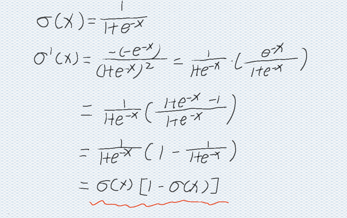
log([σ (WT ⋅ X+b)]y * [1 − σ (WT ⋅ X+b)]1 − y)
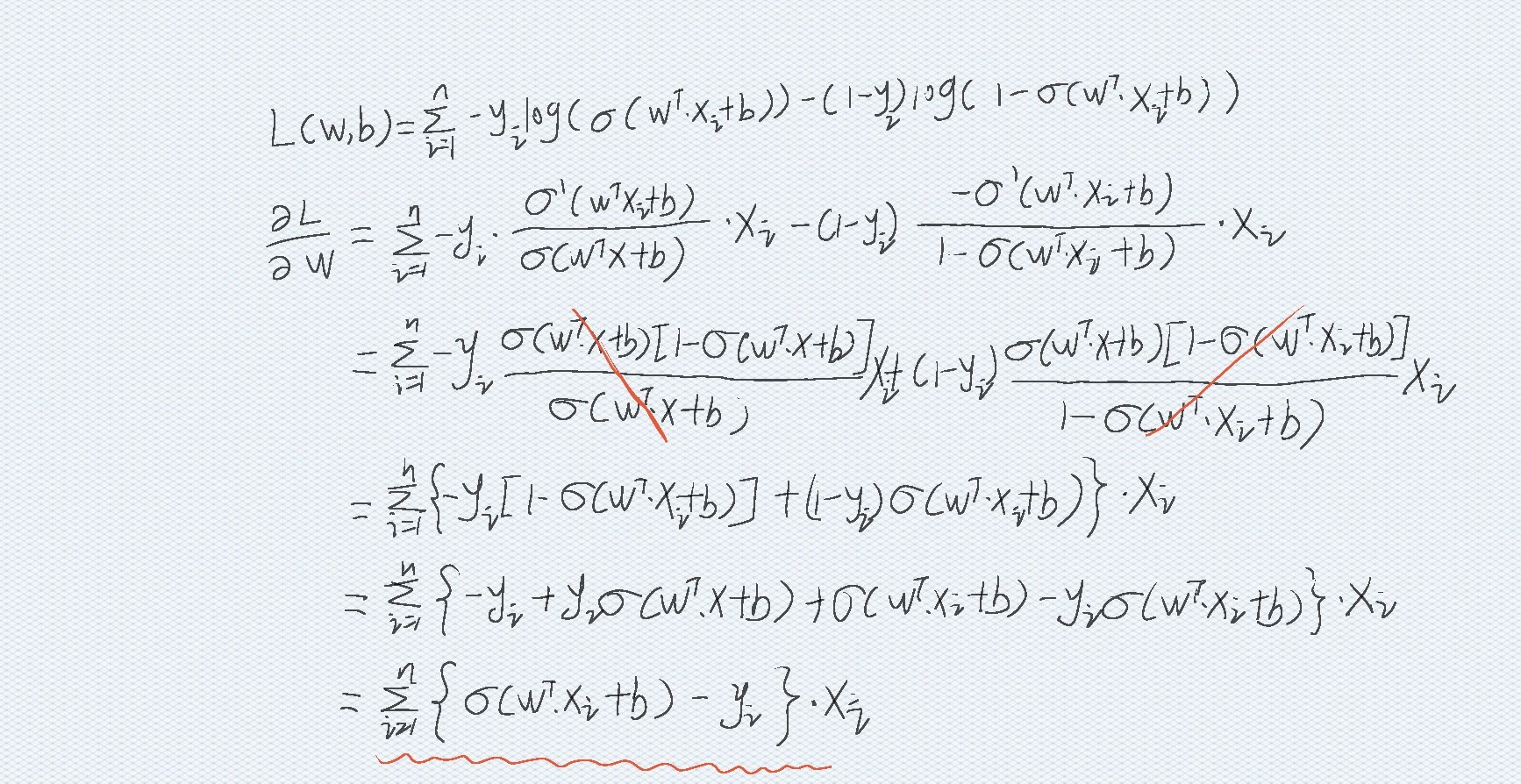
{σ (wT ⋅ x i + b) − yi} ⋅ xi
The same can be obtained
∂L(w,b)∂b=∑i=1n{σ(wT⋅xi+b)−yi} \frac{\partial L(w,b)}{\partial b} =\sum_{i=1}^n \{\sigma(w^T \cdot x_i+b )-y_i\}∂b∂L(w,b)=i=1∑n{σ(wT⋅xi+b)−yi}
Now just let the derivative be zero.
as long as
∑i=1n{σ(wT⋅xi+b)−yi}⋅xi=0 \sum_{i=1}^n \{\sigma(w^T \cdot x_i+b )-y_i\}\cdot x_i=0i=1∑n{σ(wT⋅xi+b)−yi}⋅xi=0
Well
How about that
These are all vectors and sigma functions. What should I do?
As long as ideas do not slide, there are more ways than difficulties.
1.4. Minimum value by gradient descent method
Gradient descent method is an iterative method to find the extreme value. Here is a brief introduction.
This entry is reviewed by the compilation and application project of "popular science China" Science Encyclopedia.
The original meaning of gradient is a vector (vector), which means that the directional derivative of a function at the point gets the maximum value along the direction, that is, the function changes fastest along the direction (the direction of the gradient) at the point, and the change rate is the maximum (the modulus of the gradient).
The direction of the gradient is the direction of the fastest descent of the function. For convex functions, as long as the gradient is always found, the minimum point can be reached. As shown in the figure below.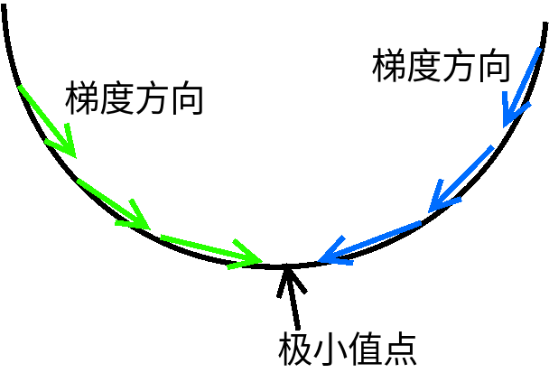
The formula is as follows
{Wt+1=Wt−η∗∑i=1n∂L(w,b)∂wbt+1=bt−η∗∑i=1n∂L(w,b)∂b\left \{\begin{array}{cc}
W_{t+1}=W_t-\eta*\sum_{i=1}^n \frac{\partial L(w,b)}{\partial w}\\
\\
b_{t+1}=b_t-\eta* \sum_{i=1}^n \frac{\partial L(w,b)}{\partial b}
\end{array}\right. ⎩⎨⎧Wt+1=Wt−η∗∑i=1n∂w∂L(w,b)bt+1=bt−η∗∑i=1n∂b∂L(w,b)
1.5. How to end the cycle - system assessment?
-
Accuracy
-
f1-measure
-
cost function
cost=−1∑i=1n{ y∗log(P(y=1∣xi))+(1−y)∗log(P(y=0∣xi )}cost = \frac {-1} { \sum _{i=1}^{n} \{~ y * log(P(y=1|x_i)) + (1 - y) * log(P(y=0|x_i~)\}}cost=∑i=1n{ y∗log(P(y=1∣xi))+(1−y)∗log(P(y=0∣xi )}−1
2. Write code now
2.1 import data
Dataset: link Extraction code: k2ug
import pandas as pd
df=pd.read_csv("corpurs/train_loan_data.csv")#Modify the file directory by yourself
#View data
prinf(df.head(5))
The output is as follows
    Loan_ID Gender Married  ... Credit_History Property_Area Loan_Status
0  LP001002   Male      No  ...            1.0         Urban           Y
1  LP001003   Male     Yes  ...            1.0         Rural           N
2  LP001005   Male     Yes  ...            1.0         Urban           Y
3  LP001006   Male     Yes  ...            1.0         Urban           Y
4  LP001008   Male      No  ...            1.0         Urban           Y
[5 rows x 13 columns]
[Finished in 2.0s]
2.1 data preprocessing
Check first. Is there any missing value?
print(df.info())
output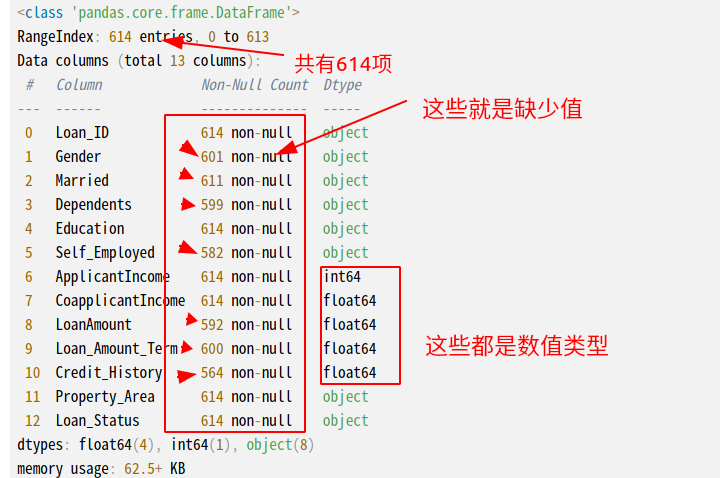 There are many missing values. But now it can't be filled in. Because there are many strings that can't be processed, we need to standardize them first. The table is as follows:
| Loan_ID | Gender | Married | Dependents | Education | Self_Employed | ApplicantIncome | CoapplicantIncome | LoanAmount | Loan_Amount_Term | Credit_History | Property_Area | Loan_Status |
|---|---|---|---|---|---|---|---|---|---|---|---|---|
| LP001002 | Male | No | 0 | Graduate | No | 5849 | 0 | 360 | 1 | Urban | Y | |
| LP001003 | Male | Yes | 1 | Graduate | No | 4583 | 1508 | 128 | 360 | 1 | Rural | N |
First replace Y and N of loan status with 1,0
Remove the unrelated column loan? ID
df.drop('Loan_ID', axis=1, inplace= True)
df.Loan_Status.replace({'Y': 0, 'N': 1}, inplace= True)
Then use one hot encoding, for example, the Gender column has two types: Male and Female.
We encode the column name as Gender_Male with a value of 1, and 0 for Male and Female respectively.
dummies=pd.get_dummies(df,drop_first=True)
print(dummies.info())
The output is as follows:
 #   Column                   Non-Null Count  Dtype
---  ------                   --------------  -----
 0   ApplicantIncome          614 non-null    int64
 1   CoapplicantIncome        614 non-null    float64
 2   LoanAmount               592 non-null    float64
 3   Loan_Amount_Term         600 non-null    float64
 4   Credit_History           564 non-null    float64
 5   Loan_Status              614 non-null    int64
 6   Gender_Male              614 non-null    uint8
 7   Married_Yes              614 non-null    uint8
 8   Dependents_1             614 non-null    uint8
 9   Dependents_2             614 non-null    uint8
 10  Dependents_3+            614 non-null    uint8
 11  Education_Not Graduate   614 non-null    uint8
 12  Self_Employed_Yes        614 non-null    uint8
 13  Property_Area_Semiurban  614 non-null    uint8
 14  Property_Area_Urban      614 non-null    uint8
The following can be supplemented with missing values
#Use simpleImputer for default value supplement.
from sklearn.impute import SimpleImputer
SimImp = SimpleImputer()
train= pd.DataFrame(SimImp.fit_transform(dummies), columns=dummies.columns)
Extract the value of the result column (loan status) in the dataset into y, and delete the loan status column in the dataset.
y=np.array(df['Loan_Status'])
train.drop('Loan_Status', inplace= True, axis= 1)
The current data table is as follows:
| ApplicantIncome | CoapplicantIncome | LoanAmount | Loan_Amount_Term | Credit_History | Gender_Male | Married_Yes | Dependents_1 | Dependents_2 | Dependents_3+ | Education_Not Graduate | Self_Employed_Yes | Property_Area_Semiurban | Property_Area_Urban |
|---|---|---|---|---|---|---|---|---|---|---|---|---|---|
| 5849.0 | 0.0 | 146.41216216216216 | 360.0 | 1.0 | 1.0 | 0.0 | 0.0 | 0.0 | 0.0 | 0.0 | 0.0 | 0.0 | 1.0 |
| 4583.0 | 1508.0 | 128.0 | 360.0 | 1.0 | 1.0 | 1.0 | 1.0 | 0.0 | 0.0 | 0.0 | 0.0 | 0.0 | 0.0 |
Now that all the data has been sorted out, the following features are extracted.
2.2 extract features
Use the original df data to see the impact of each attribute on the result.
The code is as follows:
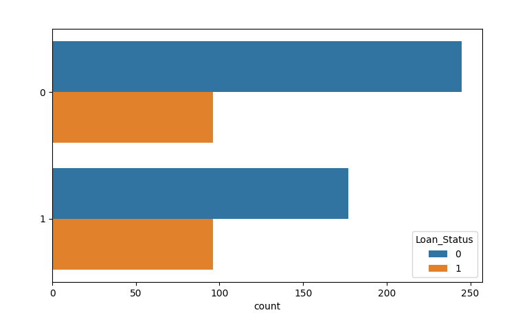
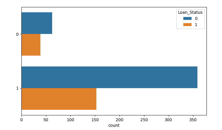
obj_cols=['Gender', 'Married','Dependents','Education','Self_Employed','Property_Area']
plt.figure(figsize=(24, 18))
for idx, cols in enumerate(obj_cols):
    plt.subplot(3, 3, idx+1)
    sns.countplot(cols, data= df, hue='Loan_Status')
plt.show()
Output results: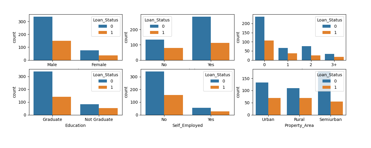 It is found that each attribute has different influence on the result. You can keep it.
Let's look at the impact of successive columns on the results. In theory, continuous data discretization should be carried out to determine the step size of each data discretization. But for the sake of simplicity, the method of visual judgment is adopted here.
- ApplicantIncome
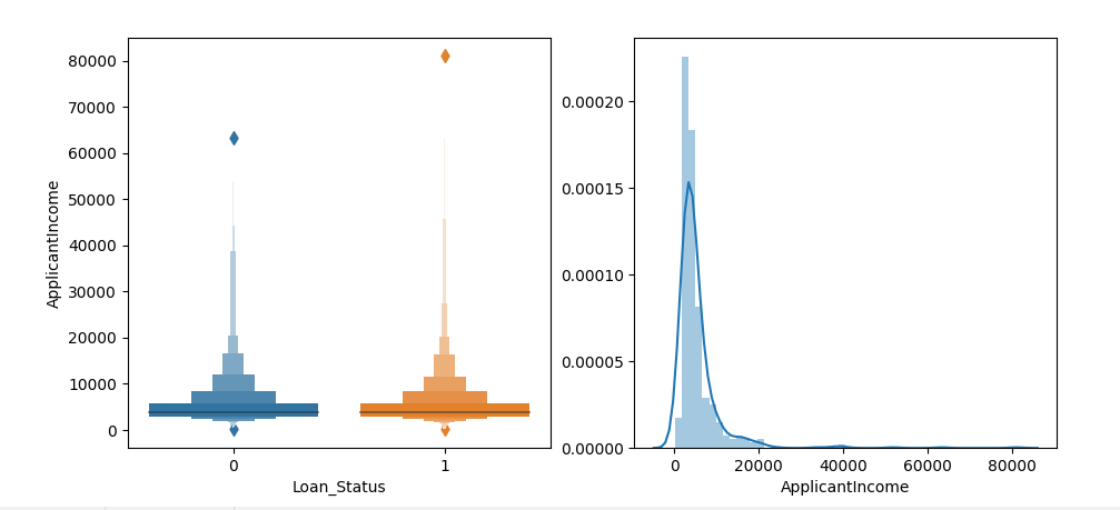 Data segmentation in median
ApplicantIncome_3850= np.where(train.ApplicantIncome <= 3850, 1, 0)
sns.countplot(y=ApplicantIncome_3850, hue=train.Loan_Status)
plt.show()
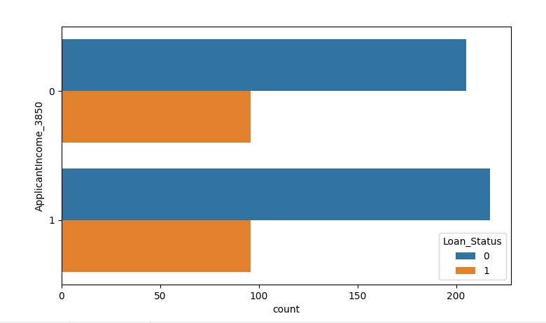 The result shows that there is no obvious classification effect, so skip this attribute first.
train.drop('ApplicantIncome', inplace= True, axis= 1)
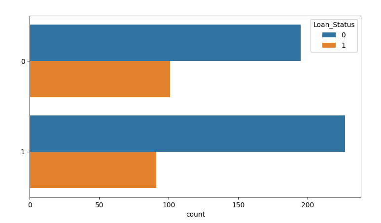
- CoapplicantIncome
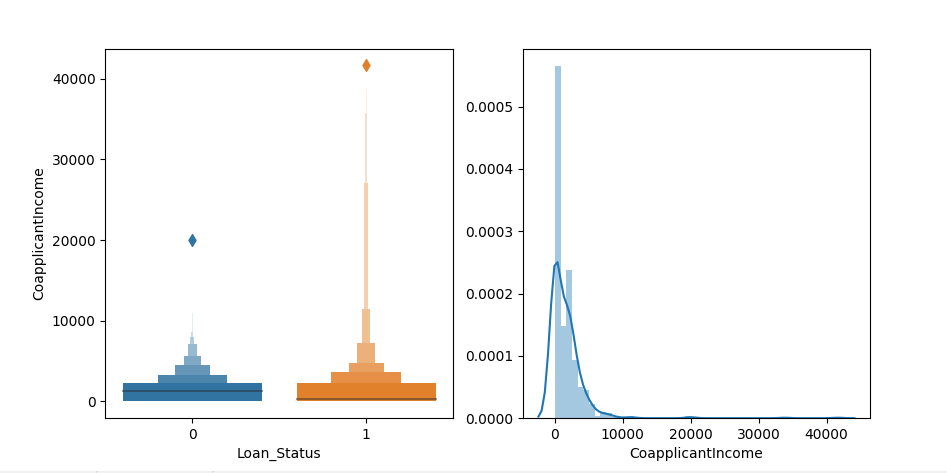
CoapplicantIncome_0= np.where(train.CoapplicantIncome == 0, 1, 0)
sns.countplot(y=CoapplicantIncome_0, hue=train.Loan_Status)
plt.show()
It can be seen from the above that no matter whether the CoapplicantIncome property is zero or not, the number of passes does not change, so this property is skipped.
train.drop('CoapplicantIncome', inplace= True, axis= 1)
- LoanAmount
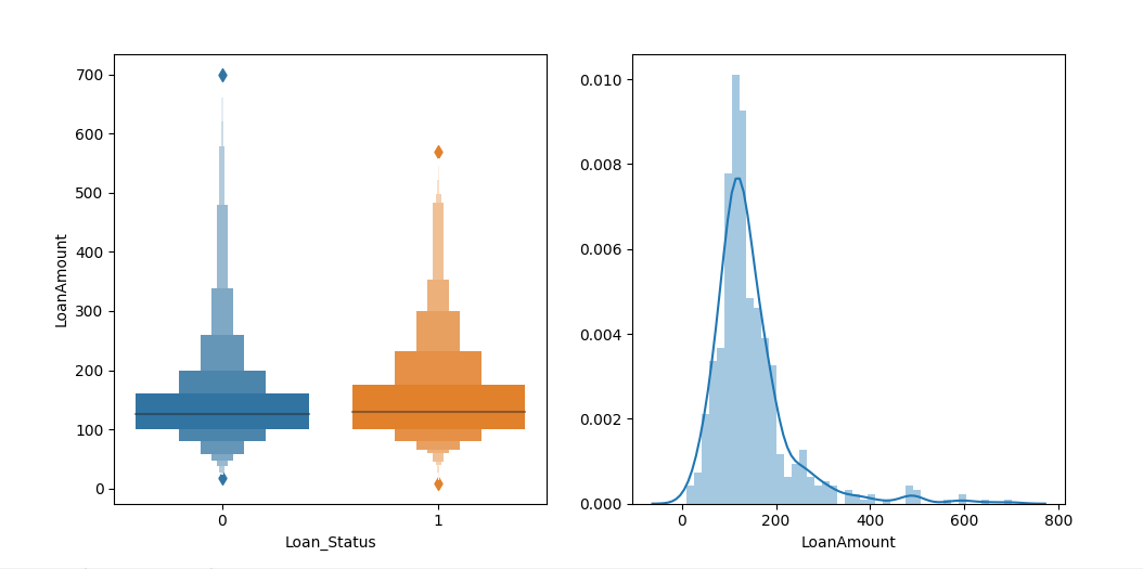
LoanAmount_130= np.where(train.LoanAmount <= 130, 1, 0)
sns.countplot(y=LoanAmount_130, hue=train.Loan_Status)
plt.show()
train.drop('LoanAmount', inplace= True, axis= 1)
- Loan_Amount_Term
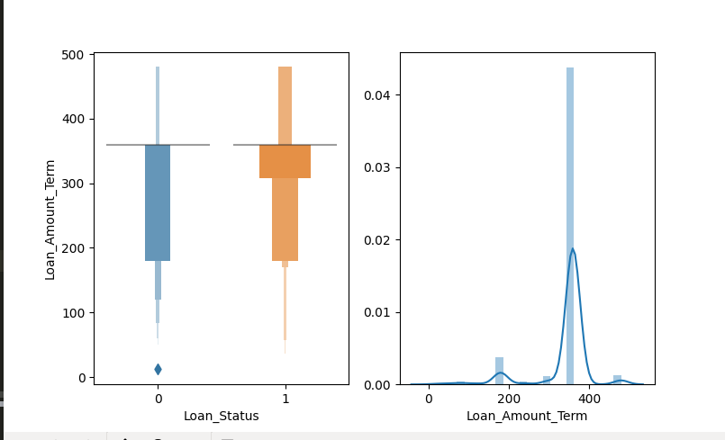
Loan_Amount_Term_360= np.where(train.Loan_Amount_Term >= 360, 1, 0)
sns.countplot(y=Loan_Amount_Term_360, hue=train.Loan_Status)
plt.show()
train['Loan_Amount_Term_360']=Loan_Amount_Term_360
train.drop('Loan_Status', inplace= True, axis= 1)
This is the end of feature extraction.
| Credit_History | Gender_Male | Married_Yes | Dependents_1 | Dependents_2 | Dependents_3+ | Education_Not Graduate | Self_Employed_Yes | Property_Area_Semiurban | Property_Area_Urban | Loan_Amount_Term_360 |
|---|---|---|---|---|---|---|---|---|---|---|
| 1.0 | 1.0 | 0.0 | 0.0 | 0.0 | 0.0 | 0.0 | 0.0 | 0.0 | 1.0 | 1.0 |
| 0.0 | 1.0 | 1.0 | 1.0 | 0.0 | 0.0 | 0.0 | 0.0 | 0.0 | 0.0 | 1.0 |
2.5 model building
Write sigmoid function
import math
def sigmoid(x):
	try:#Prevent excessive spillage
	    ans = math.exp(-x)
	except OverflowError:
	    ans = float('inf')
	return 1/(1+ans)
def logistics_regression(Max_count,train,y):

	for t in range(Max_count):
		detal=0
		temp_w=np.zeros(length).T
		for i in range(num_train):
			x=train[i]#Take out a column of data
			detal+=( sigmoid(w.dot(x)+b)-y[i])
			temp_w+=detal*x
		#Two parameters corrected
		cost+=abs(detal)
		w=w-ita*temp_w
		b=b-ita*detal
Write the test function to test the
def test(w,b,test,y):
	right=0
	for i in range(len(test)):
		x=test[i]
		res=1 if sigmoid(w.dot(x)+b)>0.5 else 0
		if res==y[i]:
			right+=1
	return right/len(test) if right != 0 else 0
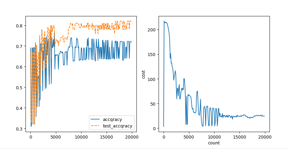
The correct rate of test at the end of training is: 82.0%
w=[-4077.22220218  1553.16884731   814.90560572   100.48750814
 -1295.03048226   461.71877025   282.46035556   919.35256087
  3025.51140312  2495.27421114 -1241.55514724]
b= -231.76993931561967
This is the result of 20000 times of training. The accuracy of test set is 82%
3. Problems to be improved:
- Discretization of continuous features
- How to adjust learning rate dynamically
- In the initial state, wt ⋅ x i + B = 0W ^ T \ cdot x ⋅ I + B =When 0wt ⋅ xi + b=0, cost is infinite.
- Details of cross entropy loss function
- Why the accuracy of test set is higher than that of test set
Reference article:
Loan Prediction-by jazeel66
Understanding of learning rate and how to adjust it
Detailed explanation of cross entropy loss function by red stone
Appendix 1: data set
Dataset: link Extraction code: k2ug
Appendix 2: source code
# loan_prediction.py
import numpy as np
import matplotlib.pyplot as plt
import seaborn as sns
from sklearn.impute import SimpleImputer
import pandas as pd
# 2.1 data import
df=pd.read_csv("corpurs/train_loan_data.csv")
# print(df.head(5))

# 2.2 data preprocessing
print(df.info())
#Remove the unimportant loan? ID column
df.drop('Loan_ID', axis=1, inplace= True)
#Replace Y and N values
df.Loan_Status.replace({'Y': 0, 'N': 1}, inplace= True)
#Use encoding
dummies=pd.get_dummies(df,drop_first=True)
# print(dummies.info())


#Use simpleImputer for default value supplement.
SimImp = SimpleImputer()
train= pd.DataFrame(SimImp.fit_transform(dummies), columns=dummies.columns)

#Take the result set y and delete the column
y=np.array(df['Loan_Status'])
train.drop('Loan_Status', inplace= True, axis= 1)

train.to_csv('train_csv.csv')

# 2.3 feature extraction


train['Loan_Status']=y

# obj_cols=['Gender',
#  'Married',
#  'Dependents',
#  'Education',
#  'Self_Employed',
#  'Property_Area']
# plt.figure(figsize=(24, 18))

# for idx, cols in enumerate(obj_cols):

#     plt.subplot(3, 3, idx+1)

#     sns.countplot(cols, data= df, hue='Loan_Status')

# ApplicantIncome|CoapplicantIncome|LoanAmount|Loan_Amount_Term|
# plt.subplot(1, 2, 1)
# sns.boxenplot(x='Loan_Status', y= 'ApplicantIncome', data= df)
# plt.subplot(1, 2, 2)
# sns.distplot(df.loc[df['ApplicantIncome'].notna(), 'ApplicantIncome'])
# plt.show()

Loan_Amount_Term_360= np.where(train.Loan_Amount_Term == 360, 1.0, 0)
# sns.countplot(y=Loan_Amount_Term_360, hue=train.Loan_Status)
# plt.show()

train['Loan_Amount_Term_360']=Loan_Amount_Term_360

train.drop('Loan_Status', inplace= True, axis= 1)


train=train.drop(['ApplicantIncome', 'Loan_Amount_Term','CoapplicantIncome', 'LoanAmount'],axis= 1)

train.info()
train.to_csv('train_csv.csv')

# 2.4 start modeling

import math
def sigmoid(x):
	try:
		ans = math.exp(-x)
	except OverflowError:
		ans = float('inf')
	return 1/(1+ans)


def test(w,b,test,y):
	right=0
	for i in range(len(test)):
		x=test[i]
		res=1 if sigmoid(w.dot(x)+b)>0.5 else 0
		if res==y[i]:
			right+=1
	return right/len(test) if right != 0 else 0


def logistics_regression(Max_count,train,y):

	length=len(train.columns)
	#Initialize w, b, η
	w,b=np.random.rand(length).T,1
	ita=0.01#Learning step η

	train=np.array(train.values)

	# Divide training set and test set
	test_data=train[-100:]
	test_y=y[-100:]
	train=train[:-100]
	y=y[:-100]

	train_count=[]#Record training times
	train_acc=[]#Record accuracy
	test_acc=[]#Record accuracy
	_cost=[]
	max_w=[]#Record the best w
	max_b=-999999#Record the best b
	max_acc=0#Record current contention rate
	num_train=len(train)
	cost=0
	for t in range(Max_count):
		detal=0
		temp_w=np.zeros(length).T
		for i in range(num_train):
			x=train[i]#Take out a column of data

			detal+=( sigmoid(w.dot(x)+b)-y[i])
			temp_w+=detal*x
		#Two parameters corrected
		cost+=abs(detal)
		w=w-ita*temp_w
		b=b-ita*detal
		#Test the effect every 100 times
		# if t%2000==0:
		# 	ita/=2
		if t%100==0:
			# a = sigmoid(w.dot(x)+b)
			# cost =1/(- y[i] * np.log(a) - (1 - y[i]) * np.log(1 - a))
			_cost.append(cost/100)
			print(f"underway{t}Secondary learning....Error:{cost/100}")
			cost=0
			right=test(w,b,train,y)
			right_1=test(w,b,test_data,test_y)
			if right_1>max_acc:
				max_acc=right_1
				max_b=b
				max_w=w
			train_count.append(t)
			train_acc.append(right)
			test_acc.append(right_1)

	df=pd.DataFrame(train_acc,index =train_count)
	df['accqracy']=train_acc
	df['count']=train_count
	df['cost']=_cost
	df['test_accqracy']=test_acc

	plt.figure(figsize=(24, 18))
	plt.subplot(1,2,1)
	sns.lineplot(data=[df['accqracy'],df['test_accqracy']])
	plt.subplot(1,2,2)
	sns.lineplot(y='cost',x='count',data=df)

	print(f"The correct rate of test at the end of training is:{max_acc*100}%")
	print(max_acc,max_w,max_b)
	plt.show()
	return max_acc,max_w,max_b

Max_count=20000#Number of tests
logistics_regression(Max_count,train,y)

