There is no standard process for data preprocessing, which is usually different for different tasks and data set attributes. Let's take a look at the common six steps to complete data preprocessing.
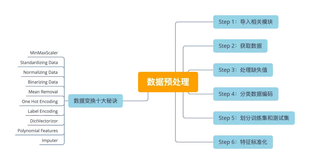
Step 1: import related modules
import numpy as np
import matplotlib.pyplot as plt
import pandas as pd

import warnings
warnings.filterwarnings("ignore")

import yfinance as yf
yf.pdr_override()
Step 2: get data
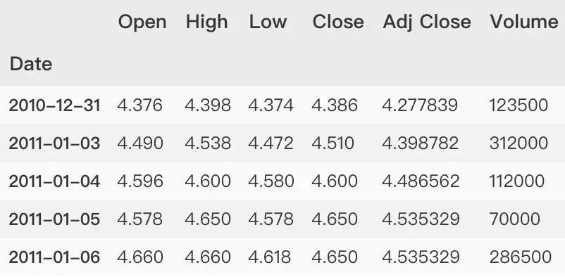
symbol = 'TCEHY'
start = '2011-01-01'
end = '2021-03-31'
dataset = yf.download(symbol,start,end)

# View data
dataset.head()
X = dataset[['Open', 'High', 'Low', 'Volume']].values
y = dataset['Adj Close'].values

Characteristic structure
dataset['Increase_Decrease'] = np.where(dataset['Volume'].shift(-1) > dataset['Volume'],1,0)
dataset['Buy_Sell_on_Open'] = np.where(dataset['Open'].shift(-1) > dataset['Open'],1,0)
dataset['Buy_Sell'] = np.where(dataset['Adj Close'].shift(-1) > dataset['Adj Close'],1,0)
dataset['Returns'] = dataset['Adj Close'].pct_change()
dataset = dataset.dropna()
dataset.head()
Step 3: Processing missing values
from sklearn.preprocessing import Imputer
imputer = Imputer(missing_values = "NaN", strategy = "mean", axis = 0)
imputer = imputer.fit(X[ : , 1:3])
X[ : , 1:3] = imputer.transform(X[ : , 1:3])
Step 4: classification data coding
from sklearn.preprocessing import LabelEncoder, OneHotEncoder
labelencoder_X = LabelEncoder()
X[ : , 0] = labelencoder_X.fit_transform(X[ : , 0])
- Create dummy variable
onehotencoder = OneHotEncoder(categorical_features = [0])
X = onehotencoder.fit_transform(X).toarray()
labelencoder_Y = LabelEncoder()
Y =  labelencoder_Y.fit_transform(Y)
Step 5: divide training set and test set
from sklearn.cross_validation import train_test_split
X_train, X_test, Y_train, Y_test = train_test_split(
         X ,
         Y ,
         test_size = 0.2,
         random_state = 0)
Step 6: feature standardization
from sklearn.preprocessing import StandardScaler
sc_X = StandardScaler()
X_train = sc_X.fit_transform(X_train)
X_test = sc_X.fit_transform(X_test)
Ten Secrets of data transformation
Data transformation [1] is to multiply each element of the data set by a constant; That is, transform every number into, where and are real numbers. Data transformation may change the distribution of data and the location of data points.
MinMaxScaler
>>> from sklearn.preprocessing import MinMaxScaler
>>> scaler=MinMaxScaler(feature_range=(0,1))
>>> rescaledX=scaler.fit_transform(X)
>>> np.set_printoptions(precision=3) # Sets the precision of the output
>>> rescaledX[0:5,:]
array([[0.009, 0.008, 0.009, 0.01 ],
       [0.01 , 0.009, 0.01 , 0.003],
       [0.01 , 0.009, 0.01 , 0.001],
       [0.01 , 0.009, 0.01 , 0.009],
       [0.01 , 0.009, 0.01 , 0.017]])
Standardizing Data
Data standardization [2] (sometimes called z-score or standard score) is a variable that has been rescaled to a mean of zero and a standard deviation of 1. For the standardized variable, the value of the value in each case on the standardized variable indicates the difference between it and the mean (or standard deviation) of the original variable.
>>> from sklearn.preprocessing import StandardScaler
>>> scaler=StandardScaler().fit(X)
>>> rescaledX=scaler.transform(X)
>>> rescaledX[0:5,:]
array([[-1.107, -1.105, -1.109, -0.652],
       [-1.102, -1.102, -1.103, -0.745],
       [-1.103, -1.1  , -1.103, -0.764],
       [-1.099, -1.099, -1.102, -0.663],
       [-1.103, -1.101, -1.105, -0.564]])
Normalizing Data
Normalized data is to scale the data to the range of 0 to 1.
>>> from sklearn.preprocessing import Normalizer
>>> scaler=Normalizer().fit(X)
>>> normalizedX=scaler.transform(X)
>>> normalizedX[0:5,:]
array([[1.439e-05, 1.454e-05, 1.433e-05, 1.000e+00],
       [4.104e-05, 4.107e-05, 4.089e-05, 1.000e+00],
       [6.540e-05, 6.643e-05, 6.540e-05, 1.000e+00],
       [1.627e-05, 1.627e-05, 1.612e-05, 1.000e+00],
       [9.142e-06, 9.222e-06, 9.082e-06, 1.000e+00]])
Binarizing Data
Binarization [3] is the process of converting the data features of any entity into binarized vectors to make the classifier algorithm more efficient. In a simple example, converting the gray scale of an image from 0-255 spectrum to 0-1 spectrum is binarization.
>>> from sklearn.preprocessing import Binarizer
>>> binarizer=Binarizer(threshold=0.0).fit(X)
>>> binaryX=binarizer.transform(X)
>>> binaryX[0:5,:]
array([[1., 1., 1., 1.],
       [1., 1., 1., 1.],
       [1., 1., 1., 1.],
       [1., 1., 1., 1.],
       [1., 1., 1., 1.]])
Mean Removal
De mean method is the process of removing the mean from each column or feature and making it zero centered.
>>> from sklearn.preprocessing import scale
>>> data_standardized=scale(dataset)
>>> data_standardized.mean(axis=0)
array([ 0.000e+00,  0.000e+00, -8.823e-17, -1.765e-16, -8.823e-17,
        8.823e-17,  6.617e-17,  1.792e-17, -2.654e-17, -7.065e-18])

>>> data_standardized.std(axis=0)
array([1., 1., 1., 1., 1., 1., 1., 1., 1., 1.])
One Hot Encoding
Heat independent coding [4] is a process of converting classification variables into a form that can be provided to ML algorithm for better prediction.
>>> from sklearn.preprocessing import OneHotEncoder
>>> encoder=OneHotEncoder()
>>> encoder.fit(X)
OneHotEncoder(categorical_features=None, categories=None,
       dtype=<class 'numpy.float64'>, handle_unknown='error',
       n_values=None, sparse=True)
Label Encoding
Label coding is applicable to data with classification variables and converting data into numbers.
- fit
>>> from sklearn.preprocessing import LabelEncoder
>>> label_encoder=LabelEncoder()
>>> input_classes=['Apple','Intel','Microsoft','Google','Tesla']
>>> label_encoder.fit(input_classes)
>>> LabelEncoder()

>>> for i,companies in enumerate(label_encoder.classes_):
...     print(companies,'-->',i)
Apple --> 0
Google --> 1
Intel --> 2
Microsoft --> 3
Tesla --> 4
- transform
labels=['Apple','Intel','Microsoft']
label_encoder.transform(labels)
array([0, 2, 3], dtype=int64)
label_encoder.inverse_transform(label_encoder.transform(labels))
array(['Apple', 'Intel', 'Microsoft'], dtype='<U9')
DictVectorizor
Word vectors are used for data with labels and numbers. In addition, word vectors can be used to extract data.
>>> from sklearn.feature_extraction import DictVectorizer
>>> companies = [{'Apple':180.25,'Intel':45.30,
                  'Microsoft':30.26,'Google':203.75,
                  'Tesla':302.18}]
>>> vec = DictVectorizer()
>>> vec.fit_transform(companies).toarray()
array([[180.25, 203.75, 45.3 , 30.26, 302.18]])- Get feature name
>>> vec.get_feature_names()
['Apple', 'Google', 'Intel', 'Microsoft', 'Tesla']
Polynomial Features
Polynomial features are used to generate polynomial features and interactive features. It also generates a new feature matrix data, which is composed of polynomial combinations of all features whose degree is less than or equal to the specified degree.
>>> from sklearn.preprocessing import PolynomialFeatures
>>> poly = PolynomialFeatures(2) # Quadratic interaction term
>>> poly.fit_transform(X)
array([[1.000e+00, 4.490e+00, 4.538e+00, ..., 2.000e+01, 1.395e+06,
        9.734e+10],
       ...,
       [1.000e+00, 7.857e+01, 7.941e+01, ..., 6.089e+03, 1.339e+08,
2.944e+12]])- Intercept term
>>> poly = PolynomialFeatures(interaction_only=True) # Do not keep intercept items
>>> poly.fit_transform(X)
array([[1.000e+00, 4.490e+00, 4.538e+00, ..., 2.029e+01, 1.416e+06,
        1.395e+06],
       ...,
       [1.000e+00, 7.857e+01, 7.941e+01, ..., 6.196e+03, 1.363e+08,
        1.339e+08]])
Imputer
Padding (e.g., filling missing values with means), which replaces missing values with the mean in the column or characteristic data
>>> from sklearn.preprocessing import Impute >>> imputer = SimpleImputer() >>> print(imputer.fit_transform(X, y)) [[4.490e+00 4.538e+00 4.472e+00 3.120e+05] ... [7.857e+01 7.941e+01 7.803e+01 1.716e+06]]