catalogue
3.2 the core of LSTM is three gate functions
It's been a while since the last RNN. On the one hand, I don't want to write. On the other hand, because other things are involved, I've been procrastinating. Today, I write LSTM, hoping to explain it from the perspective of undergraduates.
1. What is lstm
LSTM: long short term memory network (LSTM) is a kind of time cyclic neural network, which is specially designed to solve the long-term dependence problem of general RNN (cyclic neural network). All RNNs have a chain form of repetitive neural network modules.
RNN portal: Comments continue to send books. Xiaobai can understand the most easily understood RNN articles in history
RNN problem: there is the problem of gradient explosion and disappearance, which is not good for learning long-distance sentences.
Gradient disappearance: the RNN gradient disappears because the reciprocal of the tanh function of the activation function is between 0 and 1. When updating the parameters at the previous time during back propagation, when the parameter W is initialized to a number less than 1, multiple (tanh function '* W) are multiplied, which will lead to the minimum of the obtained partial derivative (the number less than 1 is multiplied), resulting in the disappearance of the gradient.
Gradient explosion: when the parameter is initialized to be large enough so that the reciprocal of tanh function multiplied by W is greater than 1, it will lead to the maximum partial derivative (multiple numbers greater than 1), resulting in gradient explosion.
In short, when the parameter is greater than 1, the n-th power of 1 will explode and approach positive infinity. When the parameter is less than 1, the n-th power of 1 will disappear and approach 0. A separate article will be written on the mathematical reasoning of back propagation
2. Network structure of lstm
The following figure is the simplest one I have seen in my study. It can be said that I understand LSTM because of this figure.
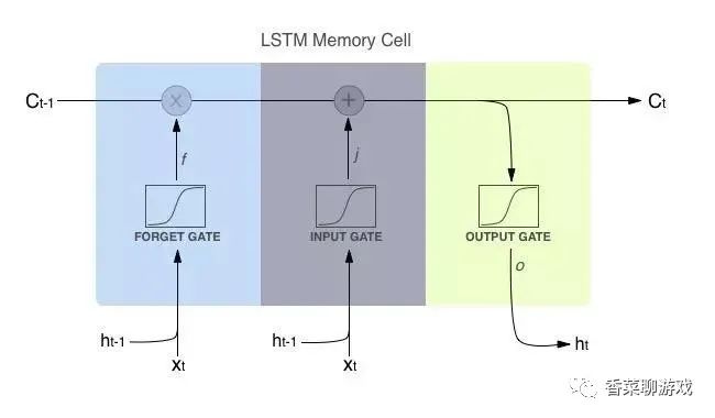
The main idea is to store information in memory cells, and memory cells in different hidden layers form a conveyor belt (red line in the figure) through a small amount of linear interaction to realize the flow of information. At the same time, a "door" structure is introduced to add or delete information in memory cells and control the flow of information.
1. Architecture diagram
I don't know anything. Look at other people's architecture
Note:
x is the multiplication of the corresponding elements in the operation matrix, so it is required that the two multiplication matrices are of the same type
+The sign represents matrix addition.
Ct-1 is the output of the current neuron
Ht-1 is the parameter of the hidden layer
It can be seen from the architecture diagram that there are mainly three gate units, forgetting gate, input gate and output gate.
The inputs of the forgetting gate and the input gate are the input Xt of the current time and the data of the previous hidden layer
The input of the output gate is the current output
3. lstm's door
The above is to understand the structure of LSTM. The details will be introduced below. Try to use popular language to help you understand. Mathematical formulas will also be attached. If you can understand it, you can understand it. If you can't understand it, it won't affect you.
First attach the classic LSTM architecture (the painting is really not good, it's too difficult to understand)
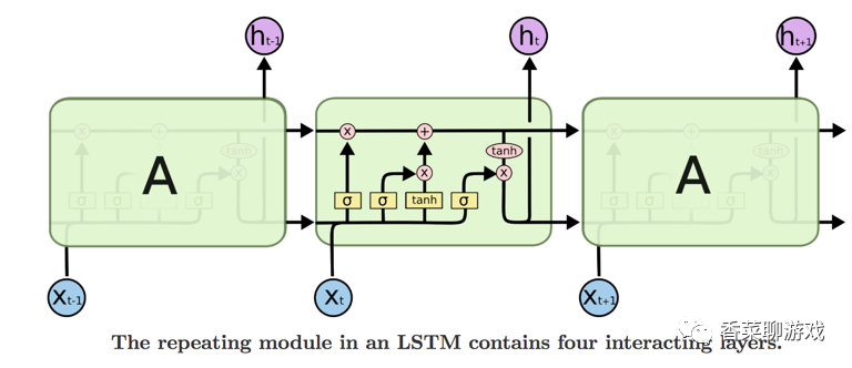
The gate represents the neural network layer. For example, tanh is not a simple tanh function in the conventional sense, but the tanh neural network layer. Pay attention to the distinction
Although the final effect is the same, it is a neural network, and the neural network layer has parameters.
3.1 description of input data
for instance:
Here we will focus on the data entered under
For example, the input is: I love Beijing Tiananmen Square
Encode the input [1,2,3,4,5,6,7] (generally, it is not encoded in this way. It is usually encoded as a word vector. This is just for illustration)
Input Xt-1 = 2, then Xt = 3, and the whole sentence is a sequence.
3.2 the core of LSTM is three gate functions
In another simple diagram, you can see that there are only two sigmod and tanh neural network layers used by the current cell
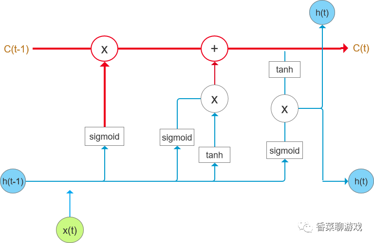
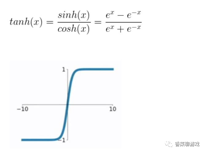
tanh neural network layer
The entered value will be kept in the range of [- 1,1],
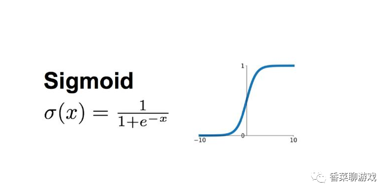
sigmod neural network layer
The input data will be converted into the interval of (0,1)
3.3 door
The forgetting gate is responsible for how much memory in the forgetting memory unit Ht-1 is saved.
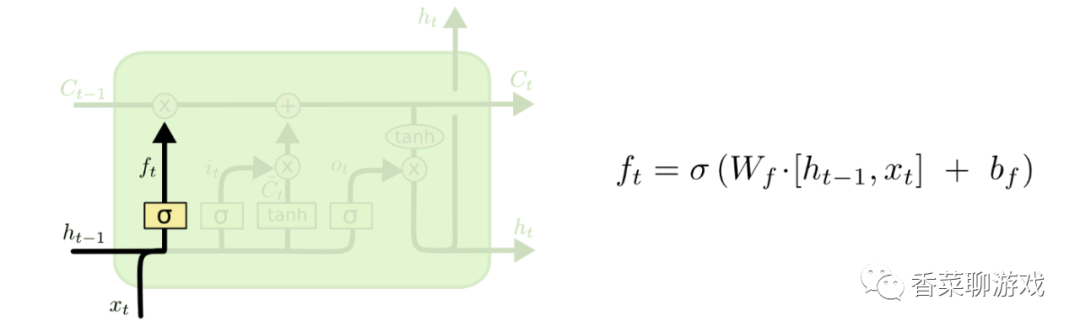
As shown in the figure: the mathematical operation is analyzed below
Ht-1 = [0.1,0.2,0.3] is a matrix with one row and three columns
Xt = [0.6,0.7,0.8] is also a matrix with one row and three columns
Then [Ht-1,Xt] = [0.1,0.2,0.3,0.6,0.7,0.8], i.e
6 represents a neural unit, and the model of the whole function is f = wx +b
Wf is the parameter of the current neural unit
bf is the offset parameter
The output of the whole neuron is all values between (0,1) through sigmoid function, such as [0.4,0.8,0.9]
3.4 input gate
The function of the input gate is to add new things to the status information
The input gate consists of two parts, and two neuron functions are used at the same time.
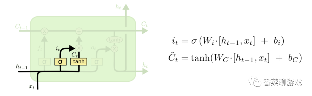
The operation of It function is similar to that of the input gate above, which is used to control the update degree of new state information
Ct is used to control the input data
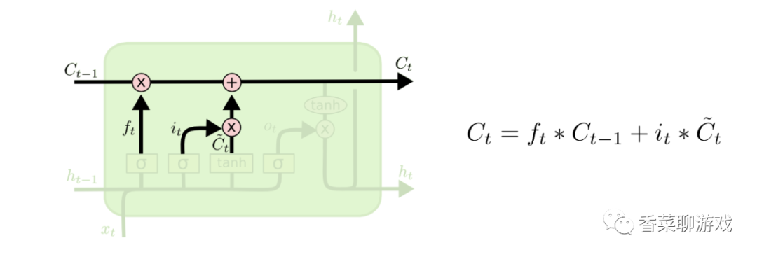
The final output result is a function of the results of the above two steps. I believe you should know what this mathematical formula means
Ct is the output of the current time
Ct-1 is the output of the last time
It is the update degree of the input door
C"t is the data of the control input
3.5 output valve
We need to determine what value to output. The output will be based on our cell state, but it is also a filtered version. First, we run a sigmoid layer to determine which part of the cell state will be output. Then, we process the cell state through tanh (get a The value between 0 and 1) and multiply it by the output of the sigmoid gate. Finally, we will only output the part of the output we determine.
The output gate is the memory of the output, that is, the accumulation in front
The output gate is also two neural units
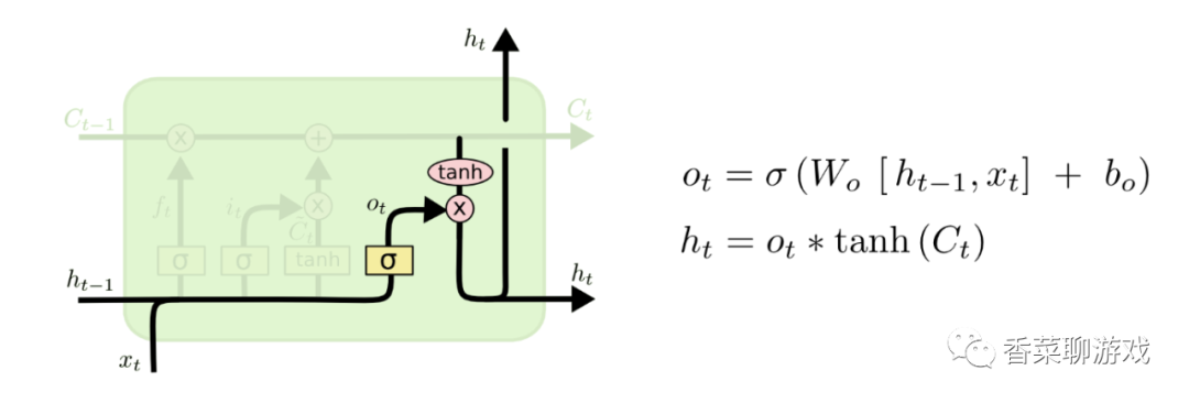
Ot is the sigmod neural unit
Ht is the tanh unit with Ct as input
4. pytorch module parameters
pytorch provides the implementation of LSTM, so let's explain the parameters below
class torch.nn.LSTM(*args, **kwargs)
Parameters are:
     input_size: characteristic dimension of x
     hidden_size: feature dimension of hidden layer
     num_layers: the number of layers of lstm hidden layer, which is 1 by default
     bias: False, then bihbih=0 and bhhbhh=0. The default is True
     batch_first: True, then the input and output data format is (batch, seq, feature)
     Dropout: except for the last layer, the output of each layer is dropout. The default is 0
     Bidirectional: True is bidirectional, lstm is False by default
input(seq_len, batch, input_size)
Parameters are:
     seq_len: sequence length, which is the sentence length in NLP. Generally, pad_sequence is used to supplement the length
     batch: the number of data pieces fed to the network each time. In NLP, it is the number of sentences fed to the network at a time
     input_size: feature dimension, and the input of the network structure defined above_ Size is consistent.
output,(ht, ct) = net(input)
     Output: the neuron output of the hidden layer in the last state
     ht: the state value of the hidden layer of the last state
     ct: the forgetting gate value of the hidden layer of the last state
5. lstm example
Required packages:
numpy ,pandas matplotlib ,pytorch
Environment installation portal: It's too late to go into the pit. Learn pytorch from scratch and build the environment step by step
Source code:
import torch
import torch.nn as nn
import torch.nn.functional
import numpy as np
import pandas as pd
import matplotlib.pyplot as plt
"""
Import data
"""
# load the dataset
flight_data = pd.read_csv('flights.csv', usecols=[1], engine='python')
dataset = flight_data.values
dataset = dataset.astype('float32')
print(flight_data.head())
print(flight_data.shape)
#Plot monthly passenger travel frequency
fig_size = plt.rcParams['figure.figsize']
fig_size[0] = 15
fig_size[1] = 5
plt.rcParams['figure.figsize'] = fig_size
plt.title('Month vs Passenger')
plt.ylabel('Total Passengers')
plt.xlabel('Months')
plt.grid(True)
plt.autoscale(axis='x',tight=True)
plt.plot(flight_data['passengers'])
plt.show()
"""
Data preprocessing
"""
flight_data.columns#Displays the data type of the column in the dataset
all_data = flight_data['passengers'].values.astype(float)#Change the data type of the passengers column to float
#Partition test set and training set
test_data_size = 12
train_data = all_data[:-test_data_size]#Except for the last 12 data, all others are retrieved
test_data = all_data[-test_data_size:]#Take the last 12 data
print(len(train_data))
print(len(test_data))
#The maximum and minimum scaler is normalized to reduce the error
from sklearn.preprocessing import MinMaxScaler
scaler = MinMaxScaler(feature_range=(-1, 1))
train_data_normalized = scaler.fit_transform(train_data.reshape(-1, 1))
#View the first 5 pieces of data and the last 5 pieces of data after normalization
print(train_data_normalized[:5])
print(train_data_normalized[-5:])
#Convert the data set to tensor, because PyTorch model is trained with tensor, and convert the training data into input sequence and corresponding label
train_data_normalized = torch.FloatTensor(train_data_normalized).view(-1)
#view is equivalent to resize in numpy, and the parameter represents the dimensions of different dimensions of the array;
#If the parameter is - 1, the dimension of this dimension is inferred by the machine. If there is no - 1, all parameters in the view must be consistent with the total number of elements in the tensor
#Define create_ inout_ The sequences function receives the original input data and returns a list of tuples.
def create_inout_sequences(input_data, tw):
inout_seq = []
L = len(input_data)
for i in range(L-tw):
train_seq = input_data[i:i+tw]
train_label = input_data[i+tw:i+tw+1]#Forecast time_ First value after step
inout_seq.append((train_seq, train_label))#inout_ The data in SEQ is constantly updated, but the total amount is only tw+1
return inout_seq
train_window = 12#Set the sequence length of training input to 12, similar to time_step = 12
train_inout_seq = create_inout_sequences(train_data_normalized, train_window)
print(train_inout_seq[:5])#Production data set transformation results
"""
be careful:
create_inout_sequences The returned tuple list consists of a sequence,
Each sequence has 13 data, including 12 data set( train_window)+ 13th data( label)
The first sequence consists of the first 12 data, and the 13th data is the label of the first sequence.
Similarly, the second sequence starts with the second data and ends with the 13th data, while the 14th data is the label of the second sequence, and so on.
"""
"""
establish LSTM Model
Parameter Description:
1,input_size:The corresponding and characteristic quantity, in this case, is 1, i.e passengers
2,output_size:Number of prediction variables and number of data labels
2,hidden_layer_size:The characteristic number of the hidden layer, that is, the number of neurons in the hidden layer
"""
class LSTM(nn.Module):#Note that the Module initials need to be capitalized
def __init__(self, input_size=1, hidden_layer_size=100, output_size=1):
super().__init__()
self.hidden_layer_size = hidden_layer_size
# LSTM layer and linear layer are created, LSTM layer extracts features, and linear layer is used as the final prediction
##The LSTM algorithm accepts three inputs: the previous hidden state, the previous cell state and the current input.
self.lstm = nn.LSTM(input_size, hidden_layer_size)
self.linear = nn.Linear(hidden_layer_size, output_size)
#Initialize the hidden state and cell state C, and the hidden_cell variable contains the previous hidden state and cell state
self.hidden_cell = (torch.zeros(1, 1, self.hidden_layer_size),
torch.zeros(1, 1, self.hidden_layer_size))
# Why is the second parameter also 1
# The second parameter should represent batch_size
# Is it because the data has been segmented before?????
def forward(self, input_seq):
lstm_out, self.hidden_cell = self.lstm(input_seq.view(len(input_seq), 1, -1), self.hidden_cell)
#The output of LSTM is the hidden state ht and cell state ct of the current time step and the output lstm_out
#Modify the shape of input_seq according to the format of lstm as the input of linear layer
predictions = self.linear(lstm_out.view(len(input_seq), -1))
return predictions[-1]#Returns the last element of the predictions
"""
forward method: LSTM Input and output of layer: out, (ht,Ct)=lstm(input,(h0,C0)),among
1, Input format: lstm(input,(h0, C0))
1,input For( seq_len,batch,input_size)Formatted tensor,seq_len mean time_step
2,h0 by(num_layers * num_directions, batch, hidden_size)Formatted tensor,Initial state of hidden state
3,C0 by(seq_len, batch, input_size)Formatted tensor,Initial cell state
2, Output format: output,(ht,Ct)
1,output by(seq_len, batch, num_directions*hidden_size)Formatted tensor,Include output features h_t(originate from LSTM each t The last floor of)
2,ht by(num_layers * num_directions, batch, hidden_size)Formatted tensor,
3,Ct by(num_layers * num_directions, batch, hidden_size)Formatted tensor,
"""
#Create an object of the LSTM() class and define the loss function and optimizer
model = LSTM()
loss_function = nn.MSELoss()
optimizer = torch.optim.Adam(model.parameters(), lr=0.001)#Create optimizer instance
print(model)
"""
model training
batch-size Refers to the sample size used in one iteration;
epoch It means to go through all training data completely;
Because by default, the weight is PyTorch Neural networks are randomly initialized, so different values may be obtained.
"""
epochs = 300
for i in range(epochs):
for seq, labels in train_inout_seq:
#Clears the previous gradient value of the network
optimizer.zero_grad()#When training the model, you need to make the model in the training mode, that is, call model.train(). By default, the gradient is cumulative. You need to initialize or reset the gradient manually, and call optimizer.zero_grad()
#Initialize hidden layer data
model.hidden_cell = (torch.zeros(1, 1, model.hidden_layer_size),
torch.zeros(1, 1, model.hidden_layer_size))
#Instantiation model
y_pred = model(seq)
#Calculate the loss, back propagation gradient and update the model parameters
single_loss = loss_function(y_pred, labels)#In the training process, the forward propagation generates the output of the network and calculates the loss value between the output and the actual value
single_loss.backward()#Call loss.backward() to automatically generate the gradient,
optimizer.step()#The optimizer is executed using optimizer.step() to propagate the gradient back to each network
# View the results of model training
if i%25 == 1:
print(f'epoch:{i:3} loss:{single_loss.item():10.8f}')
print(f'epoch:{i:3} loss:{single_loss.item():10.10f}')
"""
forecast
be careful, test_input Contains 12 data,
stay for In the loop, 12 data will be used to predict the first data of the test set, and then append the predicted value to the test_inputs In the list.
In the second iteration, the last 12 data will be used as input again, a new prediction will be made, and then the new value of the second prediction will be added to the list again.
Since there are 12 elements in the test set, the loop will execute 12 times.
At the end of the cycle, test_inputs The list will contain 24 data, of which the last 12 data will be the predicted values of the test set.
"""
fut_pred = 12
test_inputs = train_data_normalized[-train_window:].tolist()#First print out the last 12 values of the data list
print(test_inputs)
#Change the model to test or validation mode
model.eval()#Set the training property to false to make the model in the test or verification state
for i in range(fut_pred):
seq = torch.FloatTensor(test_inputs[-train_window:])
with torch.no_grad():
model.hidden = (torch.zeros(1, 1, model.hidden_layer_size),
torch.zeros(1, 1, model.hidden_layer_size))
test_inputs.append(model(seq).item())
#Print the last 12 predictions
print(test_inputs[fut_pred:])
#Since the training set data is standardized, the prediction data is also standardized
#The normalized predicted value needs to be converted into the actual predicted value. It is realized through inverse_transform
actual_predictions = scaler.inverse_transform(np.array(test_inputs[train_window:]).reshape(-1, 1))
print(actual_predictions)
"""
Draw the predicted value according to the actual value
"""
x = np.arange(132, 132+fut_pred, 1)
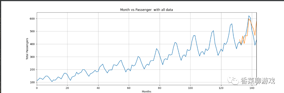
plt.title('Month vs Passenger with all data')
plt.ylabel('Total Passengers')
plt.xlabel('Months')
plt.grid(True)
plt.autoscale(axis='x', tight=True)
plt.plot(flight_data['passengers'])
plt.plot(x, actual_predictions)
plt.show()
#Draw the actual and predicted number of passengers in the last 12 months to observe the data on a larger scale
plt.title('Month vs Passenger last pred data')
plt.ylabel('Total Passengers')
plt.xlabel('Months')
plt.grid(True)
plt.autoscale(axis='x', tight=True)
plt.plot(flight_data['passengers'][-train_window:])
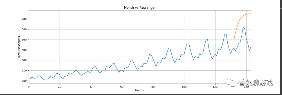
plt.plot(x, actual_predictions)
plt.show()Take a look at the results of 150 and 300 epochs I trained. It seems that the effect of 300 epochs is good, which basically simulates the trend.
Source code and data download address: https://download.csdn.net/download/perfect2011/33085064
6. Summary
The three gates of LSTM are the key points. It's easy to understand the three gates, but the introduction of many contents leads to more parameters and makes the training more difficult. Therefore, we often use GRU with the same effect as LSTM but fewer parameters to build a model with a large amount of training. Next, let's talk about GRU, an optimized or reduced version of LSTM.
The codeword is not easy. Welcome to like it, leave comments, and thank you for your support
If there is any place I do not understand, please leave a message to me or add my friend. Here is my official account.