Hough transform

In the x-y coordinates of the image, the straight line passing through the point (x_i, y_i) is expressed as y_i=k∗ x_i+b (1), where k is the slope and b is the intercept

If x_i ,y_i is regarded as a constant and K and b are regarded as variables. Formula (1) can be expressed as b = - k * x_i + y_i(2)

In this way, the representation of points (x_i, y_i) in the image coordinate space x-y is transformed into the representation in the parameter space a-b. this process is called Hough transform

Hough line transformation

Principle analysis

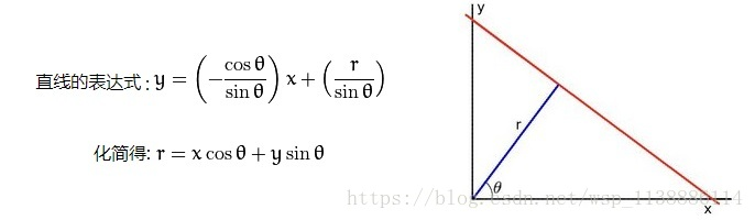
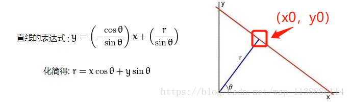
A slope and an intercept determine a straight line, but the slope may not exist, so it can be converted into Θ \Theta Θ and r r r means that the equation in parameter space can be obtained by hough transform of (x,y).

So( Θ \Theta Θ , r r r) Is a point in the parameter space, and (x,y) determines the straight line passing through the point. Passing point( Θ \Theta Θ , r r r) The more straight lines, the more points to determine these lines ( x i , y i ) (x_i, y_i) (xi, yi) the greater the likelihood of collinearity, so it is necessary to count each( Θ \Theta Θ , r r r) The number of times a straight line passes on the. This statistic corresponds to the accumulator in the recurrence code.

After obtaining the statistician, you need to determine a threshold value. If the value of the corresponding position on the statistician exceeds the threshold value, it is considered as this parameter( Θ i {\Theta}_i Θi​ , r i r_i ri) a line that can determine the linear coordinate space

According to the determined parameters( Θ i {\Theta}_i Θi​ , r i r_i ri), just make a straight line on the original drawing.

experiment

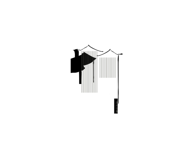
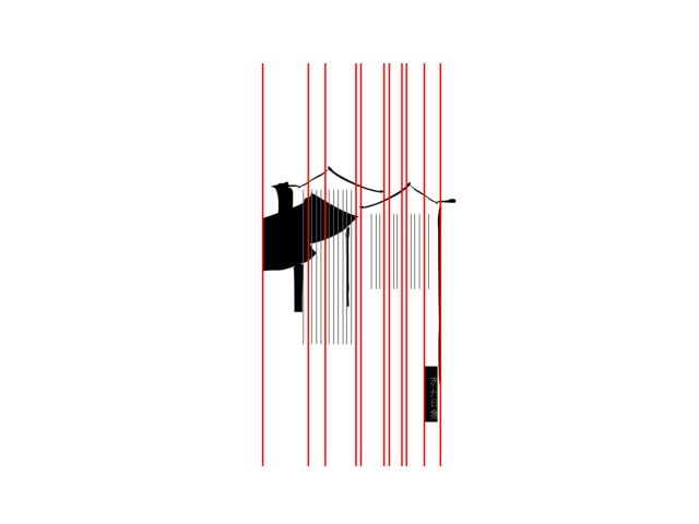
Original drawing:

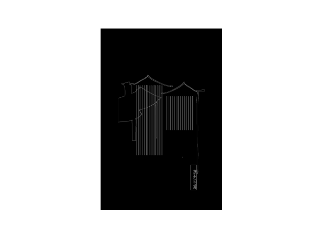
canny edge detection:

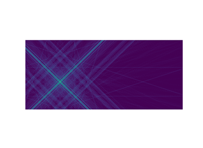
No maximum suppression:

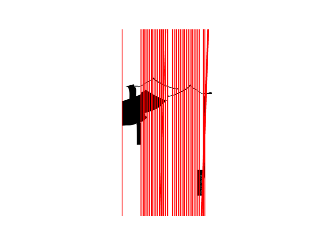
Non maximum suppression is added:

Code interpretation

Implementation of python code base

     # Implementation of hough line transform python Library
    lines = cv2.HoughLines(imgEdge, 1, np.pi / 180, 160) # 1 and np.pi/180 are the smallest units of the voting matrix, respectively
    lines1 = lines[:, 0, :]  # Extract as 2D
    for rho, theta in lines1[:]: # Take out two numbers in each line of lines
        a = np.cos(theta)
        b = np.sin(theta)
        x0 = a * rho # (x0,y0) is the constant crossing point of the parametric equation r = x * cos(theta) + y * sin(theta))
        y0 = b * rho
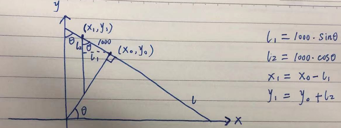
        # Using theta, rho and a known point (x0,y0) to determine the other two points on the straight line, 1000 is a random value
        x1 = int(x0 + 1000 * (-b))
        y1 = int(y0 + 1000 * (a))
        x2 = int(x0 - 1000 * (-b))
        y2 = int(y0 - 1000 * (a))
        cv2.line(img, (x1, y1), (x2, y2), (255, 0, 0), 1) # 1 is to adjust the width of the line
	plt.imshow(img, cmap="gray")
    plt.axis("off")  # Close coordinates
    plt.show()

be careful ( x 0 , y 0 ) (x_0 , y_0) (x0, y0) is the point obtained by using polar coordinates (high school knowledge)

know ( x 0 , y 0 ) (x_0 , y_0) After (x0, y0), any two points of the line can be calculated according to the principle of the following figure ( x 1 , y 1 (x_1,y_1 (x1​,y1​), ( x 2 , y 2 (x_2,y_2 (x2​,y2​):

Code recurrence:

def lineHough(imgEdge, thetaDim = None,threshold = None):
    """
    :param imgEdge: Input image after edge detection
    :param ThetaDim: Theta Number of scales on the axis (0, pi)How many copies are divided into), if it is 90, it is divided into 90 copies, and each copy is 2
    :param threshold: Threshold for voting to define whether it is a straight line
    :return: Ballot box results that meet the threshold
    """
    imgsize = imgEdge.shape
    if thetaDim == None:
        ThetaDim = 180
    MaxDist = int(np.ceil(np.sqrt(imgsize[0] ** 2 + imgsize[1] ** 2)))

    accumulator = np.zeros((ThetaDim, MaxDist))  # The range of theta is [0,pi). Here [0,pi) is linearly mapped. Similarly, Dist axis is linearly mapped

    sinTheta = [np.sin(t * np.pi / ThetaDim) for t in range(ThetaDim)]
    cosTheta = [np.cos(t * np.pi / ThetaDim) for t in range(ThetaDim)]

    for i in range(imgsize[0]):
        for j in range(imgsize[1]):
            if not imgEdge[i, j] == 0:
                for k in range(ThetaDim):
                    accumulator[k][int(round((i * cosTheta[k] + j * sinTheta[k])))] += 1

    M = accumulator.max()

    if threshold == None:
        threshold = int(M * 2.3875 / 10)
    result = np.array(np.where(accumulator > threshold))  # Thresholding
    result = result.astype(np.float64)
    result[0] = result[0] * np.pi / ThetaDim
    return result

def drawLine(line, img, color = (255, 0, 0), err = 6):
        """
    
    :param line: lineHough Returned results
    :param img: Original picture
    :param color: Color of line drawing
    :param err: Error size, adjustable
    :return: Returns the picture after the line is drawn
    """
    Cos = np.cos(line[0])
    Sin = np.sin(line[0])

    # Traverse all positions of pixels in img, and then bring the position coordinates into the parameter equation (because the two parameters can determine the straight line, meeting the equation proves that the point must be on a straight line)
    # Here. any() needs one of the two matrices to be equal. It belongs to the skill of judging the equality of two matrices
    # The error here is caused by some digital operations such as rounding and rounding when hough transform is performed, so there must be an error
    for i in range(img.shape[0]):
        for j in range(img.shape[1]):
            e = np.abs(line[1] - i * Cos - j * Sin)
            if (e < err).any():
                img[i, j] = color
    return img

Note that the drawing method here is different from that of the python library. Here, each point is traversed to judge whether each point conforms to the parameter equation, while the python library randomly selects two points and connects them to draw

Hoff circle transformation

Principle analysis

Hough gradient method

Circle detection needs to determine three parameters: (abscissa of the center of the circle, coordinates in the center of the circle, radius length). If it is calculated in three-dimensional space, the time is very long. Hough transform can be divided into two stages to reduce the dimension.

The first stage is to detect the center of the circle: if there are points on the same circumference, the gradient direction of these points should intersect the center of the circle. Therefore, the gradient of the edge points can be calculated to obtain the straight line in the gradient direction, and the intersection points of the straight lines can be accumulated. The position points with more accumulated numbers are considered as the candidate center of the circle.

The second stage detects the radius: after the position of the center of the circle is obtained, the distance from the point on the circumference to the center of the circle is equal. Therefore, the distance from each edge point to the candidate center can be calculated once, and the points of the same distance are accumulated. The distance with more accumulated numbers is considered as the candidate radius.

Determine the center of the circle

The drawing is the original image, and the right figure is the gradient direction straight line of the edge points of the original image. The bright part is the point with the most intersection times, so as to determine the center of the circle.

​

experiment

Fig. 1 is the original image, Fig. 2 is the image after canny extracting the edge, Fig. 3 is the straight line in the gradient direction of the edge point, and Fig. 4hough circle detection result

Code interpretation:

Implementation of python code base

gray = cv2.cvtColor(img, cv2.COLOR_RGB2GRAY)
cv2.waitKey(0)
# Parameters: Gray: input gray image; solution method; ratio of image pixel resolution to parameter spatial resolution; center of detected circle; minimum distance between (x,y) coordinates; param1: gradient value method for processing edge detection;
# param2: accumulator threshold. The smaller the threshold, the more circles are detected; the minimum size of the radius in pixels; the maximum size of the radius in pixels
circles = cv2.HoughCircles(gray, cv2.HOUGH_GRADIENT, 1, 100, param1 = 150,
                           param2=30, minRadius=350, maxRadius=600)
circle = circles[0, :, :] # Extract as 2D
circle = np.uint16(np.around(circle))
for i in circle[:]:
    cv2.circle(img, (i[0], i[1]), i[2], (0,0,255),5)
    cv2.circle(img, (i[0], i[1]), 2, (0, 0, 255), 10) # The radius takes two pixels, which is equivalent to adjusting the thickness of the center of the circle. The last parameter is thickness
    plt.imshow(img)
    plt.axis('off')
    plt.show()

Disadvantages: the function contains many parameters. Finally, the quality of circle detection is too correlated with the parameters, and the parameters to be adjusted in each picture are often far from each other

Code reproduction

def AHTforCircles(edge,center_threhold_factor = None,score_threhold = None,min_center_dist = None,minRad = None,maxRad = None,center_axis_scale = None,radius_scale = None,halfWindow = None,max_circle_num = None):
    if center_threhold_factor == None:
        center_threhold_factor = 10.0
    if score_threhold == None:
        score_threhold = 15.0
    if min_center_dist == None:
        min_center_dist = 80.0
    if minRad == None:
        minRad = 0.0
    if maxRad == None:
        maxRad = 1e7*1.0
    if center_axis_scale == None:
        center_axis_scale = 1.0
    if radius_scale == None:
        radius_scale = 1.0
    if halfWindow == None:
        halfWindow = 2
    if max_circle_num == None:
        max_circle_num = 6
    min_center_dist_square = min_center_dist**2


    sobel_kernel_y = np.array([[-1.0, -2.0, -1.0], [0.0, 0.0, 0.0], [1.0, 2.0, 1.0]])
    sobel_kernel_x = np.array([[-1.0, 0.0, 1.0], [-2.0, 0.0, 2.0], [-1.0, 0.0, 1.0]])
    # The gradients in the x and y directions are obtained respectively
    edge_x = convolve(sobel_kernel_x, edge, [1,1,1,1], [1,1])
    edge_y = convolve(sobel_kernel_y, edge, [1,1,1,1], [1,1])


    center_accumulator = np.zeros((int(np.ceil(center_axis_scale*edge.shape[0])),int(np.ceil(center_axis_scale*edge.shape[1]))))
    k = np.array([[r for c in range(center_accumulator.shape[1])] for r in range(center_accumulator.shape[0])])
    l = np.array([[c for c in range(center_accumulator.shape[1])] for r in range(center_accumulator.shape[0])])
    minRad_square = minRad**2
    maxRad_square = maxRad**2
    points = [[],[]] # Subscript of pixel position stored as edge and point gradient not 0
    # ((1,1), (1,1)): the front (1,1) is filled with rows, the first 1 is filled above edge_x, the second 1 is filled below edge_x, and the following (1,1) is the same
    edge_x_pad = np.pad(edge_x,((1,1),(1,1)),'constant')
    edge_y_pad = np.pad(edge_y,((1,1),(1,1)),'constant')
    Gaussian_filter_3 = 1.0 / 16 * np.array([(1.0, 2.0, 1.0), (2.0, 4.0, 2.0), (1.0, 2.0, 1.0)])
    # Vote according to gradient direction
    for i in range(edge.shape[0]):
        for j in range(edge.shape[1]):
            if not edge[i,j] == 0:
                dx_neibor = edge_x_pad[i:i+3,j:j+3]
                dy_neibor = edge_y_pad[i:i+3,j:j+3]
                dx = (dx_neibor*Gaussian_filter_3).sum()
                dy = (dy_neibor*Gaussian_filter_3).sum()
                if not (dx == 0 and dy == 0): # dx and dy are both 0. They are definitely not points on the circumference and can be excluded
                    t1 = (k/center_axis_scale-i)
                    t2 = (l/center_axis_scale-j)
                    t3 = t1**2 + t2**2
                    # Why do you find it here? t3 is the gradient of all edge points, 512 * 512, and temp is the bool matrix of [512512],
                    # Center_calculator [temp] + = 1 directly adds and subtracts the entire matrix
                    temp = (t3 > minRad_square)&(t3 < maxRad_square)&(np.abs(dx*t1-dy*t2) < 1e-4) #
                    center_accumulator[temp] += 1
                    points[0].append(i)
                    points[1].append(j)

    M = center_accumulator.mean()
    # for i in range(center_accumulator.shape[0]):
    #     for j in range(center_accumulator.shape[1]):
    #         neibor = \
    #             center_accumulator[max(0, i - halfWindow + 1):min(i + halfWindow, center_accumulator.shape[0]),
    #             max(0, j - halfWindow + 1):min(j + halfWindow, center_accumulator.shape[1])]
    #         if not (center_accumulator[i,j] >= neibor).all():
    #             center_accumulator[i,j] = 0
    #                                                                     Non maximum suppression
    # Distribution of circle center on the original drawing
    plt.imshow(center_accumulator)
    plt.axis('off')
    cwd = os.getcwd()
    saveFile = Path(cwd,"image/hough")
    plt.savefig(str(Path(saveFile, "circleImg")))
    plt.show()

    center_threshold = M * center_threhold_factor # The threshold value is obtained by using the mean value
    possible_centers = np.array(np.where(center_accumulator > center_threshold))  # Thresholding


    sort_centers = []
    for i in range(possible_centers.shape[1]):
        sort_centers.append([])
        sort_centers[-1].append(possible_centers[0,i])
        sort_centers[-1].append(possible_centers[1, i])
        sort_centers[-1].append(center_accumulator[sort_centers[-1][0],sort_centers[-1][1]])
    # Finally, each list in sort_centers is [pixel matrix x, pixel matrix y, number of votes]
    sort_centers.sort(key=lambda x:x[2],reverse=True) # Sort according to the number of votes, from large to small

    centers = [[],[],[]]
    points = np.array(points)
    for i in range(len(sort_centers)): # After determining the center of the circle, determine the radius. The radius here is a one-dimensional vector, because only the size of r needs to be determined, while the center_accumulator needs to determine two values, so it is a two-dimensional vector
        radius_accumulator = np.zeros( # The maximum value of radius statistical matrix is diagonal
            (int(np.ceil(radius_scale * min(maxRad, np.sqrt(edge.shape[0] ** 2 + edge.shape[1] ** 2)) + 1))),dtype=np.float32)
        if not len(centers[0]) < max_circle_num:
            break
        iscenter = True
        for j in range(len(centers[0])):
            d1 = sort_centers[i][0]/center_axis_scale - centers[0][j]
            d2 = sort_centers[i][1]/center_axis_scale - centers[1][j]
            if d1**2 + d2**2 < min_center_dist_square:
                iscenter = False
                break

        if not iscenter:
            continue
        # temp is the distance from each point in points to the center of the candidate circle
        temp = np.sqrt((points[0,:] - sort_centers[i][0] / center_axis_scale) ** 2 + (points[1,:] - sort_centers[i][1] / center_axis_scale) ** 2)
        temp2 = (temp > minRad) & (temp < maxRad) #temp is a vector
        temp = (np.round(radius_scale * temp)).astype(np.int32)
        for j in range(temp.shape[0]):
            if temp2[j]:
                radius_accumulator[temp[j]] += 1 # Points at this distance + 1
        for j in range(radius_accumulator.shape[0]):
            if j == 0 or j == 1:
                continue
            if not radius_accumulator[j] == 0: # np.log(j) is e ^ J, and log is the logarithm with E as the base, which feels a little normalized
                radius_accumulator[j] = radius_accumulator[j]*radius_scale/np.log(j) #radius_accumulator[j]*radius_scale/j
        score_i = radius_accumulator.argmax(axis=-1) #Which position has the largest value
        if radius_accumulator[score_i] < score_threhold: # Compared with the threshold, if it is less than the threshold, it is not judged as the center of the circle
            iscenter = False

        if iscenter:
            centers[0].append(sort_centers[i][0]/center_axis_scale)
            centers[1].append(sort_centers[i][1]/center_axis_scale)
            # Here should be the radius, but why did you return the position of the maximum radius_accumulator?
            # kang: because the length of radius_accumulator is 0-diagonal, it stores the number of occurrences at each position, so score_i is the corresponding radius
            centers[2].append(score_i/radius_scale)


    centers = np.array(centers)
    centers = centers.astype(np.float64)

    return centers

Analysis: sobel operator is used to calculate the gradient here, and the solution process is much slower than direct library adjustment

reference material:

https://zengdiqing.blog.csdn.net/article/details/86104053
https://www.bilibili.com/video/BV1bb411b7VQ