TushareID: 469107
Hello, everyone. The python assignment sharing in this issue is: how to use Tuhare's opts optimization algorithm to calculate the optimal portfolio of SSE 50 (of course, there are two restrictions: the first is the SSE 50 portfolio in a specific period of time, and the second is the stock price data in a specific historical period)

First step
Get relevant information on tushare
This step was clearly mentioned in the last assignment, so it will not be repeated this time. Only the relevant codes will be posted and explained accordingly.

#Withdrawal of constituent shares of SSE 50
pro = ts.pro_api('Yours tushare token')
date_start_50=int(input('SSE 50 component screening start period (8 digits):'))
date_end_50=int(input('SSE 50 component screening end period (8 digits):'))
df=pro.index_weight(index_code='000016.SH', start_date=date_start_50, end_date=date_end_50)
df=df.iloc[:,[0,1]]
#df.rename(columns={'index_code':'index','con_code':'code'},inplace=True)

1. In the code snippet above, date_start_50 and date_end_50 is the time period for selecting 50 constituent stocks of Shanghai Stock Exchange. Why add this time period? This is because the constituent stocks of SSE 50 have been updated. Here, I recommend that you choose one month, such as 20210101-20210201
2. Among them, iloc chose the code of SSE 50 and the code of component stocks, which you will know as soon as you try.

date_start_history=int(input('Stock selection start period according to historical data (8 bits):'))
date_end_history=int(input('Stock selection end period according to historical data (8 bits):'))
future_start=int(input('Verify the start period of the optimal combination (8 bits):'))
future_end=int(input('Verify the end period of the optimal combination (8 bits):'))

In the above code slice, the four types actually select the historical data and test section data for optimizing and calculating the optimal weight,
history is historical data and future is forecast data.

Step 2
Cleaning and sorting of data

#Data conversion and cleaning
len_df=len(df)#Measure the length of df, which will be used when selecting subscript in the lower cycle
#The following is how to obtain and process index data
df_index=pro.index_daily(ts_code='399300.SZ', start_date=date_start_history, end_date=date_end_history,fields='trade_date,pct_chg')#Get index data
df_index['trade_date']=df_index['trade_date'].astype('str')#Convert to time series-1
df_index['trade_date']=pd.to_datetime(df_index['trade_date'])#Convert to time series-2
df_index=df_index.sort_values('trade_date',ascending=True)
#The following is the stock data of component stocks
daily_trade=pro.daily(ts_code=df.iloc[4,1], start_date=date_start_history, end_date=date_end_history,fields='trade_date,close')
#Note that we chose a stupid method to get the stock price data, but we think it is very useful, that is, we traverse the component stock codes one by one and then get the data
for i in range(1,len_df):
    daily_trade1=pro.daily(ts_code=df.iloc[i,1], start_date=date_start_history, end_date=date_end_history,fields='close')
    daily_trade[df.iloc[i,1]]=daily_trade1#Change the name of close in the previous columns to the stock code, because it is convenient for us to deal with it below
daily_trade.rename(columns={'close':df.iloc[0,1]},inplace=True)#After aggregation, the closing price of the first column of stocks has not changed the name of columns, so it needs to be changed to the first column
daily_trade['trade_date']=daily_trade['trade_date'].astype('str')
daily_trade['trade_date']=pd.to_datetime(daily_trade['trade_date'])
daily_trade=daily_trade.fillna(method='pad',axis=0)#Fill the Nan data with the previous data
daily_trade=daily_trade.sort_values('trade_date',ascending=True)
print(daily_trade)#At this time, the stock data of the historical period is obtained

Step 3
Calculate the relevant values, such as variance, mean, rate of return, etc

#Calculation of logarithmic return of constituent stocks
data=daily_trade.set_index('trade_date')
r=np.log(data/data.shift(1))#The shift method is to move smoothly to the next column
r=r.dropna()#When calculating the yield, the first line is null. Delete the first line
print('Data sheet after income calculation',r)
#print(r.describe())#Description data

#Processing of component stock data
#Calculate the average return of component stocks based on historical data
mean_history_array=[]
for i in range(0,50):
    mm=np.mean(r.iloc[:,i])#50 component stocks, 50 average
    mean_history_array.append(mm)
print('The average yield of constituent stocks is',mean_history_array)
#Calculate the standard deviation of historical data return of component stocks
std_history_array=[]
for i in range(0,50):
    dd=np.std(r.iloc[:,i])#50 component stocks, 50 standard deviations
    std_history_array.append(dd)
print('The standard deviation of component stock return is',std_history_array)
#Processing of index data
#Calculate the average return of the index historical data
hs_ret_mean=np.mean(df_index.iloc[:,1])
hs_ret_std=np.std(df_index.iloc[:,1])
print('The average index return is',hs_ret_mean)
print('The standard deviation of index return is',hs_ret_std)

Step 4 - the most critical
Start opt optimization

#opt optimization
#Elements for preparing for optimization: objective function -- historical average rate of return of portfolio
from scipy.optimize import minimize
def RET(weights):    #objective function 
    weights=np.array(weights)
    return-np.dot(mean_history_array,weights)
#The following parameters will be used below, so be sure to
delta_s=0.5#Set it yourself
l=np.ones(50)#An array of all 1
n=50#50 targets

For the above delta_s coefficient. This coefficient represents how many times the risk taken is the data of SSE 50, which is set by yourself

cons=({'type':'eq','fun':lambda x:np.dot(x,l)-1},#The combined weight is equal to one
      {'type':'ineq','fun':lambda x:np.dot(mean_history_array,x)-hs_ret_mean},#Yield greater than 0
      {'type':'ineq','fun':lambda x:hs_ret_std-delta_s*np.dot(std_history_array,x)})#Variance greater than 0
bnds=tuple((0,1) for x in range(n))
x0=n*[1./n]#initial value
opts=minimize(RET,x0,method='SLSQP',bounds=bnds,constraints = cons)
print('Optimal solution combination state',opts.success)
print('Optimal solution',opts.x)

1. cons =... These lines of code represent three constraints for optimization: the first constraint is that the sum of weights is 0, the second constraint is that the income calculated according to the calculated optimal weight is greater than the income of SSE 50, and the third constraint is that the variance of the combination reconstructed according to the optimal weight is less than the variance of SSE 50, where the variance represents risk.
2. x0=n*[1./n], the meaning of this line of code is to attach an initial value to the optimal weight to be calculated and let it be calculated on the basis of the initial value. Here we give equal weight.
3. bnds=tuple((0,1) for x in range(n)). What I need to explain is that the change of line code represents that the weight cannot be less than 0, that is, short selling is not allowed, which is more in line with China's market situation.
4. Here we also need to remind you that the argument of this method can only be in the form of array, which also explains why we use the point multiplication form of np.dot in the constraints of cons.

#Add the weight to the previous df dataset
#opts.x=round(opts.x,4)
df=df.drop(columns={'index_code'})
df['weight']=np.array(opts.x)#Combine the stock code with the calculated weight
df=df.sort_values('weight',ascending=False)
df=df.iloc[:4,:]
print('Top four heavyweight stocks selected according to specific requirements',df)

The above code prints the top four weights calculated by the optimization algorithm. We will build a combination according to the four stocks and their corresponding weights.

Step 5
Calculation of comprehensive rate of return

#Comprehensive income is calculated at price
r_weight=data[df.iloc[:,0]]#Take the names of the first four stocks of the weight
len_weight1=len(df)#Count of weighted stocks filtered out
len_weight2=len(daily_trade)#Calculate len_ Length of weight1
r_weight['profit']=0
for i in range(len_weight2-1):
    r_weight.iloc[i+1,-1]=((((r_weight.iloc[i+1,0]-r_weight.iloc[0,0])/r_weight.iloc[0,0])*df.iloc[0,1]+
                          ((r_weight.iloc[i+1,1]-r_weight.iloc[0,1])/r_weight.iloc[0,1])*df.iloc[1,1]+
                          ((r_weight.iloc[i+1,2]-r_weight.iloc[0,2])/r_weight.iloc[0,2])*df.iloc[2,1]+
                          ((r_weight.iloc[i+1,3]-r_weight.iloc[0,3])/r_weight.iloc[0,3])*df.iloc[3,1])*100)
print('Print the table after calculating the weighted comprehensive rate of return (historical data)',r_weight)

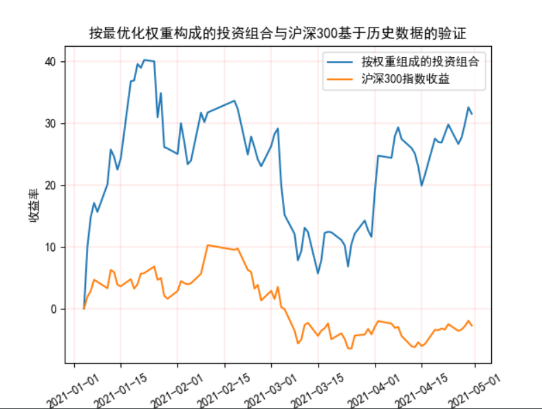
The above is to build the portfolio by weight according to the selected stocks.
How do we measure this combination? The method we adopt here is to calculate the return of the stock relative to the first day of the test date in a given test period, and calculate a total return weighted by weight.

#Get index return
df_index_price=pro.index_daily(ts_code='399300.SZ', start_date=date_start_history, end_date=date_end_history,fields='trade_date,close')
df_index_price['trade_date']=df_index_price['trade_date'].astype('str')
df_index_price['trade_date']=pd.to_datetime(df_index_price['trade_date'])
df_index_price=df_index_price.sort_values('trade_date',ascending=True)

Here is to obtain the daily price of the index. We will use a formula to solve the calculation of the yield when drawing below: ((df_index_price.iloc[:,1]-df_index_price.iloc[0,1])/df_index_price.iloc[0,1])*100)

Step 6
Visualization of historical returns

#Plot of historical returns
fig, ax = plt.subplots()
x=r_weight.index # Create the value range of x
y=r_weight.iloc[:,4]
ax.plot(x,y,label='Portfolio by weight')
x1=x
y1=(((df_index_price.iloc[:,1]-df_index_price.iloc[0,1])/df_index_price.iloc[0,1])*100)
ax.plot(x1,y1,label='CSI 300 index return')
ax.set_xlabel('date') #Set X-axis name x label
ax.set_ylabel('Yield') #Set Y-axis name y label
ax.set_title('Portfolio formed by optimal weight and verification of CSI 300 based on historical data') #Set the drawing name to Simple Plot
ax.legend()
plt.grid(color='r',linestyle='-',linewidth=0.1)
plt.xticks(rotation=30)
plt.show()

Step 7
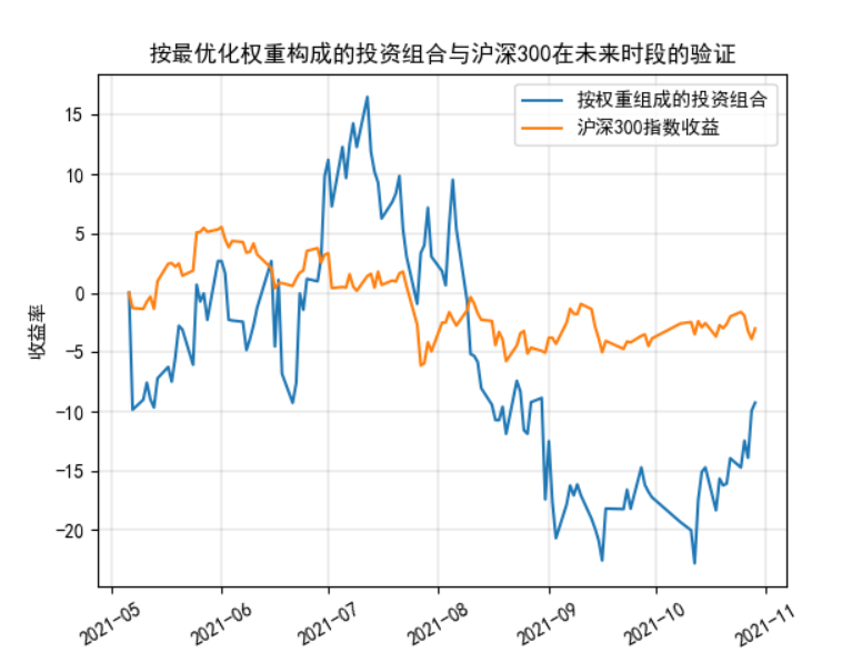
Visualization of the yield performance of the portfolio over a given test period
The principle is as above and will not be repeated

#Obtain and process validation data
df_weight=len(df)
future_weight=pro.daily(ts_code=df.iloc[0,0], start_date=future_start, end_date=future_end,fields='trade_date,close')
for i in range(1,df_weight):
    future_weight1=pro.daily(ts_code=df.iloc[i, 0], start_date=future_start, end_date=future_end,fields='close')
    future_weight[df.iloc[i,0]]=future_weight1
future_weight.rename(columns={'close':df.iloc[0,0]},inplace=True)
future_weight['trade_date']=future_weight['trade_date'].astype('str')
future_weight['trade_date']=pd.to_datetime(future_weight['trade_date'])
future_weight=future_weight.sort_values('trade_date',ascending=True)
future_weight=future_weight.set_index('trade_date')
#calculation
len_futureweight=len(future_weight)#Calculate future_ Length of weight
future_weight['profit_future']=0
for i in range(len_futureweight-1):
    future_weight.iloc[i+1,4]=((((future_weight.iloc[i+1,0]-future_weight.iloc[0,0])/future_weight.iloc[0,0])*df.iloc[0,1]+
                          ((future_weight.iloc[i+1,1]-future_weight.iloc[0,1])/future_weight.iloc[0,1])*df.iloc[1,1]+
                          ((future_weight.iloc[i+1,2]-future_weight.iloc[0,2])/future_weight.iloc[0,2])*df.iloc[2,1]+
                          ((future_weight.iloc[i+1,3]-future_weight.iloc[0,3])/future_weight.iloc[0,3])*df.iloc[3,1])*100)
print('Print the table after calculating the weighted comprehensive rate of return (validation data)',future_weight)
#Index future yield
df_index_future=pro.index_daily(ts_code='399300.SZ', start_date=future_start, end_date=future_end,fields='trade_date,close')
df_index_future['trade_date']=df_index_future['trade_date'].astype('str')
df_index_future['trade_date']=pd.to_datetime(df_index_future['trade_date'])
df_index_future=df_index_future.sort_values('trade_date',ascending=True)
#Plot of yield for future validation
fig, ax = plt.subplots()
x=future_weight.index # Create the value range of x
y=future_weight.iloc[:,-1]
ax.plot(x,y,label='Portfolio by weight')
x1=x
y1=(((df_index_future.iloc[:,1]-df_index_future.iloc[0,1])/df_index_future.iloc[0,1])*100)
ax.plot(x1,y1,label='CSI 300 index return')
ax.set_xlabel('date') #Set X-axis name x label
ax.set_ylabel('Yield') #Set Y-axis name y label
ax.set_title('Portfolio formed by optimal weight and verification of CSI 300 in the future') #Set the drawing name to Simple Plot
ax.legend()
plt.grid(color='black',linestyle='-',linewidth=0.1)
plt.xticks(rotation=30)
plt.show()

##################################################
The visualization results are as follows:


Relevant printing results are as follows:
**1. * * optimal solution combination state True

**2. * * optimal solution [3.83526119e-17 1.00000000e+00 8.09702244e-18 0.00000000e+00
2.47812608e-17 0.00000000e+00 0.00000000e+00 1.66389183e-17
5.24283153e-18 0.00000000e+00 0.00000000e+00 3.41244807e-17
1.37008501e-17 0.00000000e+00 1.89124936e-17 1.13316871e-18
0.00000000e+00 0.00000000e+00 0.00000000e+00 0.00000000e+00
0.00000000e+00 2.11767906e-18 0.00000000e+00 9.20435272e-18
5.67522288e-18 0.00000000e+00 1.66899995e-17 0.00000000e+00
1.90103020e-17 1.45697203e-17 7.48313719e-18 0.00000000e+00
0.00000000e+00 1.28748978e-17 1.22315014e-17 0.00000000e+00
0.00000000e+00 0.00000000e+00 1.58535270e-17 1.55481270e-16
2.38965369e-17 3.03270803e-18 0.00000000e+00 2.19269047e-15
3.13257514e-17 2.78092624e-17 0.00000000e+00 3.41097203e-18
0.00000000e+00 0.00000000e+00]

**3. * * top four heavyweight stocks selected according to specific requirements
con_code weight
1 603501.SH 1.000000e+00
43 600036.SH 2.192690e-15
39 600196.SH 1.554813e-16
0 603986.SH 3.835261e-17

**4. * * print the table after calculating the weighted comprehensive rate of return (historical data)
603501.SH 600036.SH 600196.SH 603986.SH profit
trade_date
2021-01-04 230.05 43.17 52.97 74.85 0.000000
2021-01-05 253.06 42.18 52.60 72.80 10.002173
2021-01-06 264.00 44.15 53.81 72.31 14.757661
2021-01-07 269.36 45.90 52.24 72.95 17.087590
2021-01-08 266.00 46.60 52.37 71.18 15.627038
... ... ... ... ... ...
2021-04-26 291.26 52.07 49.48 49.64 26.607259
2021-04-27 293.78 52.07 48.68 49.13 27.702673
2021-04-28 298.96 51.76 53.55 49.23 29.954358
2021-04-29 304.92 53.28 54.76 51.62 32.545099
2021-04-30 302.51 52.70 60.24 49.93 31.497501

[79 rows x 5 columns]
Print the table after calculating the weighted comprehensive rate of return (validation data)
603501.SH 600036.SH 600196.SH 603986.SH profit_future
trade_date
2021-05-06 293.15 53.67 54.22 187.38 0.000000
2021-05-07 264.26 54.18 54.65 177.95 -9.855023
2021-05-10 266.72 53.90 60.12 169.46 -9.015862
2021-05-11 270.95 53.84 63.14 166.05 -7.572915
2021-05-12 266.82 53.69 63.21 170.01 -8.981750
... ... ... ... ... ...
2021-10-25 249.97 54.59 51.29 152.60 -14.729661
2021-10-26 256.59 55.30 50.91 158.01 -12.471431
2021-10-27 252.39 54.52 49.73 157.56 -13.904145
2021-10-28 264.00 54.22 49.72 164.30 -9.943715
2021-10-29 266.00 53.97 50.00 169.51 -9.261470