Machine Learning Linear Discrimination Criterion and Linear Classification Programming Practice

Posted by ilovetoast on Fri, 05 Nov 2021 20:14:16 +0100

1. Linear Discrimination Criterion (LDA)

1.1 What is LDA?

Unlike PCA variance maximization theory, linear discriminant analysis (LDA) is a generalization of Fisher's linear discriminant method, which uses Statistics，pattern recognition And machine learning methods, trying to find a linear combination of the characteristics of two types of objects or events to be able to characterize or distinguish them. The resulting combination can be used as a linear classifier or, more often, to reduce the dimensionality of subsequent classifications so that the same type of data is as compact as possible and the different classes of data are as dispersed as possible. Therefore, the LDA algorithm is a supervised machine learning algorithm. At the same time, LDA has two assumptions:

(1) The original data is classified according to the mean of the sample.

(2) Data of different classes have the same covariance matrix.

Of course, in practice, it is impossible to satisfy these two assumptions. However, LDA generally works well when the data is mainly distinguished by means.

The basic idea is to project the original data to a low-dimensional space, to aggregate data of the same class as much as possible, and to disperse data of different classes as much as possible.

** Calculation steps: **

Calculates the d-dimensional mean vectors for different types of data in a dataset.
Computes the dispersion matrix, including the interspecific and intra-class dispersion matrices.
Compute the eigenvectors e1,e2,..., ed of the scatter matrix and their corresponding eigenvalues λ 1, λ 2,..., λ d.
The eigenvectors are sorted in descending order according to the size of the eigenvalues, and then the eigenvectors corresponding to the first k largest eigenvalues are selected to form a d × K-dimensional matrix - that is, each column is a eigenvector.
With this d × The k-dimensional eigenvector matrix transforms the sample into a new subspace. This step writes the matrix multiplication Y=X × W. X is n × d-dimensional matrix, representing n samples; y is n after transformation to subspace × K-dimensional sample.

1.2 Sklearn implements LDA algorithm

Import Package

import matplotlib.pyplot as plt
import pandas as pd
import numpy as np
# Import a large number of Sklearn library related packages
from sklearn.linear_model import LogisticRegression
from sklearn.discriminant_analysis import LinearDiscriminantAnalysis as LDA
from sklearn.preprocessing import StandardScaler
from sklearn.model_selection import train_test_split
from matplotlib.colors import ListedColormap

Define Visualization Functions

#Visualization Functions
def plot_decision_regions(x, y, classifier, resolution=0.02):
    markers = ['s', 'x', 'o', '^', 'v']
    colors = ['r', 'g', 'b', 'gray', 'cyan']
    cmap = ListedColormap(colors[:len(np.unique(y))])
    x1_min, x1_max = x[:, 0].min() - 1, x[:, 0].max() + 1
    x2_min, x2_max = x[:, 1].min() - 1, x[:, 1].max() + 1
    xx1, xx2 = np.meshgrid(np.arange(x1_min, x1_max, resolution), np.arange(x2_min, x2_max, resolution))
    z = classifier.predict(np.array([xx1.ravel(), xx2.ravel()]).T)
    z = z.reshape(xx1.shape)
    plt.contourf(xx1, xx2, z, alpha=0.4, cmap=cmap)
 
    for idx, cc in enumerate(np.unique(y)):
        plt.scatter(x=x[y == cc, 0],
                    y=x[y == cc, 1],
                    alpha=0.6,
                    c=cmap(idx),
                    edgecolor='black',
                    marker=markers[idx],
                    label=cc)

Fit data

#Dataset Source
data = pd.read_csv('https://archive.ics.uci.edu/ml/machine-learning-databases/wine/wine.data',header=None)

#Cutting datasets
#x data
#y label
x, y = data.iloc[:, 1:].values, data.iloc[:, 0].values

#Divide training and test sets by 8:2 ratio
x_train, x_test, y_train, y_test = train_test_split(x, y, test_size=0.2, stratify=y, random_state=0)

#Standardized unit variance
sc = StandardScaler()
x_train_std = sc.fit_transform(x_train)
x_test_std = sc.fit_transform(x_test)

lda = LDA(n_components=2)
lr = LogisticRegression()

#train
x_train_lda = lda.fit_transform(x_train_std, y_train)
#test
x_test_lda = lda.fit_transform(x_test_std, y_test)
#fitting
lr.fit(x_train_lda, y_train)

Show results

# Drawing height and width, pixels
plt.figure(figsize=(6, 7), dpi=100)  
plot_decision_regions(x_train_lda, y_train, classifier=lr)
plt.show()

2. Linear Classification Algorithm (SVM)

2.1 What is SVM

Support Vector Machine (SVM) is a class of by Supervised learning supervised learning for data Binary Classification A generalized linear classifier whose Decision boundary Is the maximum-margin hyperplane that solves the learning sample.

SVM is a sparse and robust classifier that uses the hinge loss function to compute empirical risk and incorporates a regularization term into the solution system to optimize structural risk. SVM can pass through Kernel method Nonlinear classification is one of the common kernel learning methods.

Map the feature vectors of an instance (for example, two-dimensional) to points in space, such as the solid and hollow points in the following figure, which fall into two different categories. The goal of SVM is to draw a line that "best" distinguishes the two types of points so that if there are new points in the future, the line can also be well classified.

2.2 Sklearn Implements SVM Linear Classification Algorithm

Import related packages

import numpy as np
import matplotlib.pyplot as plt
from sklearn import datasets
from sklearn.preprocessing import PolynomialFeatures,StandardScaler
from sklearn.svm import LinearSVC
from sklearn.pipeline import Pipeline
from sklearn.svm import SVC

Loading data

#Use generated data
X, y = datasets.make_moons() 
#Show data
plt.scatter(X[y==0,0],X[y==0,1]) 
plt.scatter(X[y==1,0],X[y==1,1])
plt.show()

Modify data

#Random Noise Points, random_state is a random seed and noise is a variance
X, y = datasets.make_moons(noise=0.15,random_state=520) 

#Show processed data
plt.scatter(X[y==0,0],X[y==0,1]) 
plt.scatter(X[y==1,0],X[y==1,1])
plt.show()

Define Functions

#Nonlinear SVM classification, when degree is 0 for linear
def PolynomialSVC(degree,C=1.0):
    return Pipeline([
        ("poly",PolynomialFeatures(degree=degree)),#Generate Polynomial
        ("std_scaler",StandardScaler()),#Standardization
        ("linearSVC",LinearSVC(C=C))#Finally generate svm
    ])

#Draw decision boundary
def plot_decision_boundary(model, axis):
    x0, x1 = np.meshgrid(
        np.linspace(axis[0], axis[1], int((axis[1]-axis[0])*100)).reshape(-1,1),
        np.linspace(axis[2], axis[3], int((axis[3]-axis[2])*100)).reshape(-1,1)
    )
    X_new = np.c_[x0.ravel(), x1.ravel()]
    
    y_predict = model.predict(X_new)
    zz = y_predict.reshape(x0.shape)
    
    from matplotlib.colors import ListedColormap
    custom_cmap = ListedColormap(['#EF9A9A','#FFF59D','#90CAF9'])    
    plt.contourf(x0, x1, zz, linewidth=5, cmap=custom_cmap)

#kernel function
def PolynomialKernelSVC(degree,C=1.0):
    return Pipeline([
        ("std_scaler",StandardScaler()),
        ("kernelSVC",SVC(kernel="poly")) # poly represents polynomial characteristics
    ])

#Gaussian Kernel Function
def RBFKernelSVC(gamma=1.0):
    return Pipeline([
        ('std_scaler',StandardScaler()),
        ('svc',SVC(kernel='rbf',gamma=gamma))
    ])

Linear Processing

#Linear processing, c=1
poly_svc = PolynomialSVC(degree=1,C=1)
poly_svc.fit(X,y)
plot_decision_boundary(poly_svc,axis=[-1.5,2.5,-1.0,1.5])
plt.scatter(X[y==0,0],X[y==0,1]) 
plt.scatter(X[y==1,0],X[y==1,1])
plt.show()

#Linear processing, c=500
poly_svc = PolynomialSVC(degree=1,C=500)
poly_svc.fit(X,y)
plot_decision_boundary(poly_svc,axis=[-1.5,2.5,-1.0,1.5])
plt.scatter(X[y==0,0],X[y==0,1]) 
plt.scatter(X[y==1,0],X[y==1,1])
plt.show()

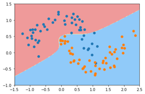
Nonlinear processing

#Nonlinear processing
poly_kernel_svc = PolynomialSVC(degree=10,C=1)
poly_kernel_svc.fit(X,y)
plot_decision_boundary(poly_kernel_svc,axis=[-1.5,2.5,-1.0,1.5])
plt.scatter(X[y==0,0],X[y==0,1]) 
plt.scatter(X[y==1,0],X[y==1,1])
plt.show()

#Nonlinear processing
poly_kernel_svc = PolynomialSVC(degree=10,C=100)
poly_kernel_svc.fit(X,y)
plot_decision_boundary(poly_kernel_svc,axis=[-1.5,2.5,-1.0,1.5])
plt.scatter(X[y==0,0],X[y==0,1]) 
plt.scatter(X[y==1,0],X[y==1,1])
plt.show()

Kernel Function Processing

#Kernel Function Processing
poly_kernel_svc = PolynomialKernelSVC(degree=10)
poly_kernel_svc.fit(X,y)
plot_decision_boundary(poly_kernel_svc,axis=[-1.5,2.5,-1.0,1.5])
plt.scatter(X[y==0,0],X[y==0,1]) 
plt.scatter(X[y==1,0],X[y==1,1])
plt.show()

#Kernel Function Processing
poly_kernel_svc = PolynomialKernelSVC(degree=50)
poly_kernel_svc.fit(X,y)
plot_decision_boundary(poly_kernel_svc,axis=[-1.5,2.5,-1.0,1.5])
plt.scatter(X[y==0,0],X[y==0,1]) 
plt.scatter(X[y==1,0],X[y==1,1])
plt.show()

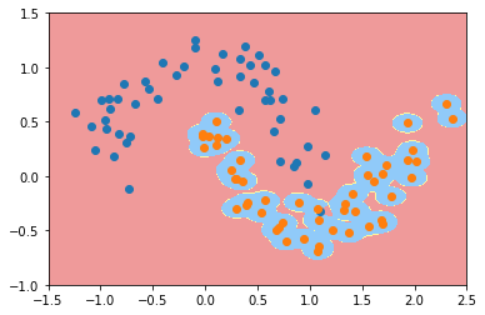
Gaussian Kernel Function Processing

#The Gaussian kernel processing parameter is 2
svc = RBFKernelSVC(2)
svc.fit(X,y)
plot_decision_boundary(svc,axis=[-1.5,2.5,-1.0,1.5])
plt.scatter(X[y==0,0],X[y==0,1]) 
plt.scatter(X[y==1,0],X[y==1,1])
plt.show()

#Gauss kernel processing parameter 20
svc = RBFKernelSVC(20)
svc.fit(X,y)
plot_decision_boundary(svc,axis=[-1.5,2.5,-1.0,1.5])
plt.scatter(X[y==0,0],X[y==0,1]) 
plt.scatter(X[y==1,0],X[y==1,1])
plt.show()

#The Gauss kernel processing parameter is 200
svc = RBFKernelSVC(100)
svc.fit(X,y)
plot_decision_boundary(svc,axis=[-1.5,2.5,-1.0,1.5])
plt.scatter(X[y==0,0],X[y==0,1]) 
plt.scatter(X[y==1,0],X[y==1,1])
plt.show()

3. Summary

LDA: Assume that the data is normally distributed. If groups have different covariance matrices, the distribution of all groups is the same, and LDA becomes quadratic discriminant analysis. LDA is the best discriminator when all assumptions are actually met. By the way, QDA is a non-linear classifier.

SVM: Summarizes the optimal separation hyperplane (OSH). OSH assumes that all groups are completely separable and SVM uses "relaxation variables" to allow some degree of overlap between groups. SVM does not assume data at all, which means it is a very flexible approach. On the other hand, flexibility often makes interpreting the results of SVM classifiers more difficult than LDA.

SVM classification is an optimization problem and LDA has a resolving solution. The optimization problem of SVM has dual and original formulas, which enable users to optimize the number of data points or variables according to the most feasible method on the data. SVM can also use the kernel to convert a SVM classifier from a linear classifier to a non-linear classifier. Search for "SVM Kernel Tips" using your favorite search engine to learn how SVM uses the kernel to convert parameter spaces.

LDA uses the entire dataset to estimate the covariance matrix, so some are prone to outliers. SVM is optimized on a subset of the data that are those data points on the delimited margin. The data points used for optimization are called support vectors because they determine how the SVM distinguishes groups to support classification.

That is, LDA is generated and SVM is distinguishable.