Original link: http://tecdat.cn/?p=24191
In this article, I will focus on an example of the inference probability given a short data sequence. I will first introduce the theory of how to use Bayesian method for expectation reasoning, and then implement the theory in Python so that we can deal with these ideas. In order to make the article easier to understand, I will only consider a small group of candidate probabilities. I can minimize the mathematical difficulty of reasoning and still get very good results, including a priori, likelihood and a posteriori graphs.
Specifically, I will consider the following situations:
- The computer program outputs a random string of 1 and 0. For example, an example output might be:

- The goal is to infer the program used to generate D 0 of The probability of. We use the symbol p0 Represents 0 The probability of. Of course, this also means 1 The probability of must be p1=1 − p0.
- As mentioned above, we only consider a set of candidate probabilities. Specifically, the candidate p0=0.2,0.4,0.6,0.8 is used for the above data sequence. How do we choose wisely among these probabilities and how sure are we of the results?
probability
My starting point is to write the probability of the sequence, just as I know the probability of 0 or 1. Of course, I don't know these probabilities - finding them is our goal - but it's a priori useful. For example, the probability of our sample data series does not need to specify the value of p0, which can be written as:
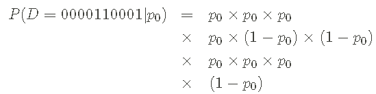
I use p1=1 − p0 to write the probability of p0. I can also write the above probability in a more compact way:
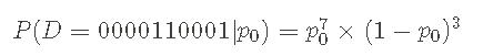
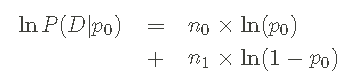
The form of probability given above is called Bernoulli process . I can also write this probability in a very general way, rather than specifically about Data Series D or probability p0, such as:
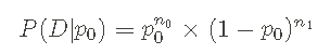
n0 and n1 represent the number of 0 and 1 in the data series.
By replacing the relevant counts and probabilities, I can relate the general form to a specific example. I first calculate the likelihood values of the data series and probability given above:

As a result, I found that p0 = 0.6 was the most likely, slightly higher than p0 = 0.8. Here are a few points to note:
- I have the maximum likelihood value (among the values considered). I can provide the answer p0=0.6 and complete it.
- Sum of probability (likelihood) Not 1—— This means that I did not normalize the probability mass function (pmf) about p0 correctly, and I tried to infer the parameters. One goal of Bayesian inference is to provide a properly normalized pmf for p0, which is called a posteriori.
The ability to perform the above calculations enables me to apply Bayesian theorem well and obtain the required a posteriori pmf. Before moving on to the Bayesian theorem, I want to emphasize the general form of likelihood function again :
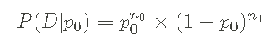
It is also useful to write down log likelihood:
Because when I create some Python code below, this form increases numerical stability. It should be clear that I use the natural (e-based) logarithm, that is, loge(x)=ln(x).
transcendental
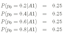
I have decided to choose p0 ∈ {0.2,0.4,0.6,0.8} as a set of probabilities I will consider. The rest is to assign a priori probability to each candidate p0 so that I can start with the correctly normalized a priori pmf. Assuming a priori equality, this is a kind of reasoning:
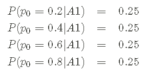
Where A1 is used to represent my assumptions. The above information constitutes a priori pmf.
Bayesian theorem and a posteriori
Next, I use Defined above likelihood and A priori pmf is used to infer the potential value of p0. That is, I will use Bayesian theorem to calculate Given likelihood and a priori Posterior pmf. A posteriori is in the form of:
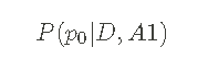
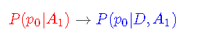
In other words, this is _ Given data sequence_ D _ And assumptions_ A1_ Yes_ p0 _ The probability of_ I can calculate a posteriori using Bayesian theorem:
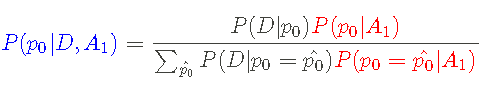
Where a priori P(p0|A1) is red, likelihood P(D|p0) is black, and a posteriori P(p0|D,A1) is blue.
This updates my p0 information from hypothesis (A1) to hypothesis + data (d, A1):
I can simplify Bayesian theorem by defining marginal likelihood function:
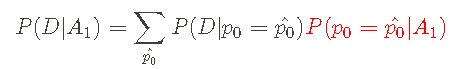
I can write the Bayesian theorem in the following form:

The posterior part should be considered as a set of equations corresponding to each candidate value of p0, just as we do for likelihood and a priori.
Finally, for the theory, I calculate the a posteriori pmf of p0. Let's start with the calculation basis (I know all the likelihood and a priori values above):
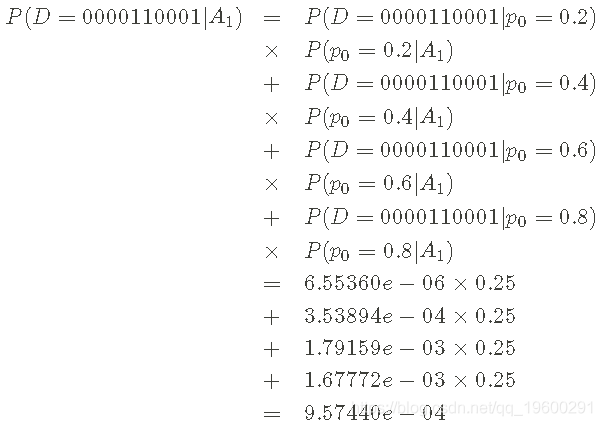
Therefore, the denominator in Bayesian theorem is equal to 9.57440e-04. Now, complete the posteriori pmf calculation.
First, 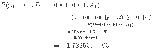
Second, 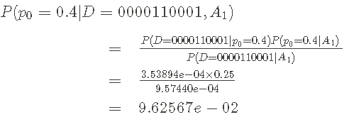
Third, 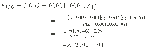
last, 
review
Before Python code, let's review the results a little. Using data and Bayesian theorem, I have learned from A priori pmf
reach Posterior pmf
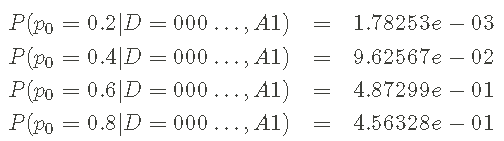
In the Bayesian setting, this a posteriori pmf is our answer to infer p0, reflecting our knowledge of the parameters of given assumptions and data. Usually people want to report a single number, but this a posteriori reflects considerable uncertainty. Some options are:
- report p0 _ Maximum a posteriori_ Value - 0.6 in this case.
- report _ Posterior mean _ Posterior median_ —— Use_ Posteriori_ pmf for calculation.
- A posteriori variance or confidence interval is included to describe the uncertainty in the estimation.
However, the report concludes that communication uncertainty is part of the work. In practice, the following figure is really helpful to complete the task. So let's leave the theory and implement these ideas in Python.
Writing reasoning code in Python
First, the code imports numpy and matplotlib. Use the ggplot style to plot.
imprt matlli.pplt as plt

#  use   mapltlb   style sheet
try:
    pl.stye.use('gglot')
First, I created a class to handle Likelihood. This class receives the data sequence and provides an interface for calculating the likelihood of a given probability p0. You can find the log likelihood equation in the method (special attention should be paid to the marginal case).
class liihd:
    def \_\_int\_\_(elf,dat):
        """binary data"""
        slff._possa(data)

    def \_pss\_a(slf,data):
        tep = \[str(x) for x in dta\]
        for s in \['0', '1'\]:
            slf.cnts\[s\] = emp.ount(s)

        if len(tmp) != sum(ef.conts.valus()):
            rase Exepon("!")

    def \_prcs\_pobites(self, p0):
        """Processing data."""
        n0 = slf.couts\['0'\]
        n1 = slf.conts\['1'\]

        if p0 != 0 and p0 != 1:
            #  example
            log_dta = n0*np.og(p0) + \
                         n1*np.log(1.-p0)
            p\_daa = np.ep(opr\_dta)
        elif p0 == 0 and n0 != 0:
            #  If it is not 0, p0 is not 0
            lordta= -np.inf
            prta = np.exp(lor_daa)
        elif p0 == 0 and n0 == 0:
            ##  Data and   p0  =  0 consistent
            logpr_data = n1*np.log(1.-p0)
            prdat = np.exp(lor_dta)
        elif p0 = 1 and n1 != 0:
            #  If   n1 is not 0   p0 is not 1
            loprta = -np.inf
            paa = np.exp(lgpaa)
        elif p0 == 1 and n1 == 0:
            ordta = n0*np.log(p0)
            prta = np.xp(lgp_dta)


    def prb(self, p0):
        """Probability of obtaining data"""
        p\_at, \_ = sef.pcrbbes(p0)

        retrn prdta

    def lo_pb(sef, p0):
        """Get log probability of data"""
        _, lp\_at = slf.p\_plie(p0)

        reurn lor_ta
Next, I'm a priori pmf creates a class . Given a list of candidate values for p0, a uniform a priori is created by default. If you need additional, you can pass a priori probabilities to override this default. Let me give an example.
class pri or:
    def \_\_ni\_\_(self, pls, pobs=Nne):
        """transcendental
           list: Permissible p0'list
           P_pos: \[Optional\]A priori probability
        """
        if p_prbs:
            #  Ensure a priori normality
            nom = sum(p_pbs.vaes())
            sel.lopct = {p:np.log(_prbs\[p\]) - \
                                np.log(nrm) for p in p_lst}
        else:
            n = len(p_is)
            sef.lo\_pict = {p:-np.log(n) for p in p\_lst}

    def \_\_iter\_\_(self):
        rturn ier(sre(slf.lopit))

    def lgpob(self, p):
        """obtain p 0 Logarithm of/A priori probability."""
        if p in sef.ogpdt:
            return sf.og_ic\[p\]
        else:
            return -np.inf

    def prob(slf, p):
        """obtain p 0 A priori probability of."""
        if p in slf.gt:
            retun np.ep(sf.o_pt\[p\])
        else:
            reurn 0.0
Finally, I construct a class for a posteriori, It uses data and an instance of a priori class to construct a posteriori pmf. The plot() method provides a very good reasoning visualization, including A priori likelihood and A posteriori graph.
Note that all posteriori calculations are done using logarithmic probabilities. This is absolutely necessary for numerical accuracy, because the probability may vary greatly and may be very small.
class posir:
    def \_\_it\_\_(slf, da ta, p ior):
        """Data: data samples as lists
        """
        sel.lod = lklio(dta)
        lf.prr = prir
        self.possior()

    def \_pocss\_ostrior(elf):
        """Use the passed data and a priori to process a posteriori."""

        nuts = {}
        deniaor = -npnf
        for p in slf.prir:
            netor\[p\] = sef.lieioo.logrob(p) + \
                            slf.riorog_rob(p)

            if nurts\[p\] != -np.inf:

                deoior = nplgxp(eoior,
                                           ners\[p\])

        #  Save the denominator in Bayesian theorem
        sef.lo_lielod = deoiato

        #  Computational posterior
        slf.ogict = {}
        for p in slf.pior:
            elf.lopct\[p\] = umros\[p\] - \
                                slf.lmllio

    def logpob(self, p):
        """Get through p Log a posteriori probability"""
        if p in self.loic:
            retrn self.ogdt\[p\]
        else:
            retrn -np.inf

    def prob(self, p):
        """Get passed p Posterior probability of"""
        if p in sl.lo_pdit:
            rtrn np.exp(sef.lct\[p\])
        else:
            rurn 0.0

    def plot(slf):
        """Draw reasoning results"""

        f, ax= plt.sbs3, 1, ise=(8, 6), hae=Tre)
        #  Obtain candidate probability from a priori
        x = \[p for p in elf.prir\]

        #  Draw a priori ob(p)   for   p   in   x\])
        ax\[0\].sem y1,inf='-, meft'', bef = -')


        #  Plot likelihood
        ax\[1\].stem(x, y, lifm= -',aerf t=ko bafmt=w')

        #  Drawing posterior
        ax\[2\].tm,y3 if='b-, mmt=bo, sefm-')
example
Let's test the code. First of all, I will copy the example we did in the theoretical example to ensure that everything is normal:
#data
data1

#  transcendental
A1 = prior(\[0.2, 0.4, 0.6, 0.8\])

#  Posteriori
pt1 = postior(da1, A1)
plot()
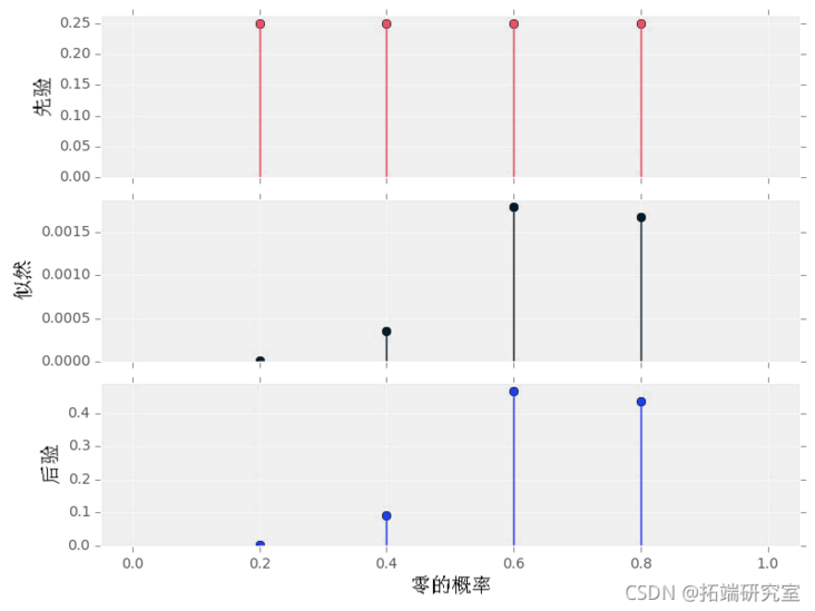
Please note how a posteriori pmf shows that both p0=0.6 and p0=0.8 have great probability - there is uncertainty! This makes sense because we have only one data series with a length of 10 and only four candidate probabilities. In addition, please note:
- The sum of all numbers in a priori and a posteriori is 1, reflecting that these are appropriate pmfs.
Next, let's consider setting a strong a priori -- a value of preference p0. Using our Python code, it is easy to see the impact of this a priori on the result a posteriori:
#  A priori-   Standardize by class
A2

#  Posteriori
po2 = ptror(data, A2)
pot()

Note the following:
- A posteriori and likelihood no longer have the same shape.
- A posteriori probability of p0=0.2,0.4_ Relative to their a priori probability_ all _ Down_ Because their likelihood for the data sequence provided is very low. In a similar way, P0 = a posteriori probability of 0.6,0.8_ Relative to their a priori probability_ Some _ Add.
Finally, let's use more candidate probabilities (here 100) and longer data sequences as an example.
#  Probability set to 0
p0 = 0.2
#  set up   rng   Seed is   four
np.andom.ed(4)
#  Generating data
da2= np.roie(\[0,1\],  p=\[p0, 1.-p0\])

#  transcendental
A3 = pir(np.aane)

#  Posteriori
ps3 = porir(daa2, A3)
plot()

Notes:
- A posteriori has a nice smooth shape - the probability I deal with looks like a continuous value.
- Note that the likelihood value (y-axis) of this data volume is very small.

Most popular insights
1.Deep learning using Bayesian Optimization in matlab
2.Implementation of Bayesian hidden Markov hmm model in matlab
3.Bayesian simple linear regression simulation of Gibbs sampling in R language
4.block Gibbs Gibbs sampling Bayesian multiple linear regression in R language
5.Bayesian model of MCMC sampling for Stan probability programming in R language
6.Python implements Bayesian linear regression model with PyMC3
7.R language uses Bayesian hierarchical model for spatial data analysis
9.Implementation of Bayesian hidden Markov hmm model in matlab