Linear model and regression

Objective: to learn a linear model to predict real value output markers as accurately as possible.

Where yi is the actual observed value and f (xi) is the regression value.
General form:

Where x=(x1, x2,..., xd) is the sample described by the d-dimensional attribute, where xi is the value of X on the ith attribute.
Vector form:

Where w=(w1, w2,..., wd) is the coefficient to be solved.

Let's take a simple example. The blog I wrote before has written about the factors that determine the evergreen tree in the singing world. x1, x2, x3... Can be used to refer to the singer's age, singing area (high, medium and low), gender (male and female), and w1, w2, w3... Are respectively
The larger the coefficient, the more important the attribute is.

Least squares and Parameter Solving

1. One dimensional data:

Considering that xi is one-dimensional data and assuming the error ei between its regression value f(xi) and the actual observation yi, the learning objectives are:

Error ei=| f(xi)-yi | can be obtained by substituting the data

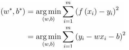
Minimize mean square error:

By deriving w and b respectively, we can get:

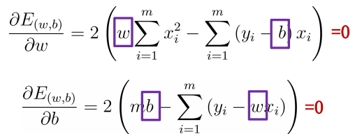
The analytical / closed form solution is obtained:

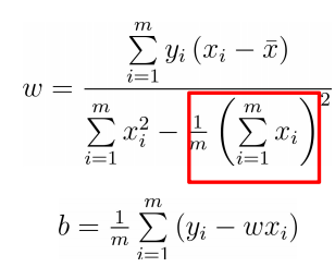
2. Multidimensional data

Multiple linear regression objectives:

Given dataset:

Integrating w and B into a vector form (w; b) data set can be expressed as:


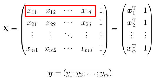
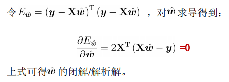
The analytical solution is as follows:

Then the linear regression model:

Maximum likelihood estimation

Maximum likelihood estimation:
Find β 0 β A value of 1 maximizes the likelihood probability

Objective function cost function:
Objective of parameter estimation optimization - > loss minimization
Log likelihood loss function

yes β Optimization algorithm: gradient descent
Find the loss function J( β) J( β) When the minimum value is obtained β

Regularization:
Penalty item is added to the loss function: the greater the parameter value, the greater the penalty – > let the algorithm minimize the parameter value
Loss function J( β):

● when model parameters β When there are too many, the loss function will be large, and the algorithm should strive to reduce it β Parameter value to minimize the loss function.
● λ Important parameters of regular term, λ The greater the penalty, the worse the model is under fitted, and on the contrary, it tends to over fit.

Logistic regression

Basic introduction

1. Regression: use a straight line (called the best fitting straight line) to fit some existing data points. This fitting process is called regression. Regression is to find the best fitting parameter set. Regression is to predict a series of continuous values, and classification is to predict a series of discrete values
Linear "regression", the purpose of the model is prediction, and the method is "regression", which is intended to "push back" (push back is to establish a linear model (including coefficients) first, and then use the training data to deduce the parameters with the minimum error.
2. Main idea: according to the existing data, a regression formula is established for the classification boundary line to classify.
3. Training classifier: find the best fitting parameter set and use the optimization algorithm.
Next, the related principles of binary output classifier are introduced.

Classification based on Logistic regression and Sigmoid function

What we need to do is a binary output classifier, that is, there are 0 and 1. The two classes that dependent variables may belong to are called negative class and positive class respectively, where 0 represents negative class and 1 represents positive class.

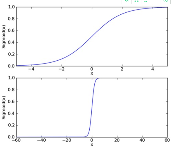
Sigmoid function formula:

In order to implement the Logistic regression classifier, we can multiply each attribute by a regression coefficient, add all the results, and substitute this synthesis into the Sigmoid function to obtain a value range of [0,1].

Determination of optimal regression coefficient based on optimization method

The Sigmoid function input is recorded as z:

Write in vector form:

Among them, vector w is the best parameter we want to find, and vector x is the input data of the classifier.

Gradient rise method of optimization algorithm

Basic idea: search along the gradient direction of a function to find the maximum value of the function.

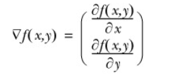
Gradient means to move ∂ f (x, y) ∂ X / ∂ X in the direction of X and ∂ f (x, y) / ∂ y in the direction of Y, where the function f (x, y) f (x, y) f (x, y) must be defined and differentiable at the point to be calculated. As shown in the following figure:

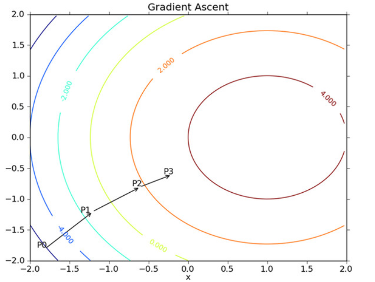
As shown in the figure above, the gradient rising algorithm will re estimate the moving direction after reaching each point. Starting from P0, after calculating the gradient of this point, the function will move to the next point P1 according to the gradient. At P1, the gradient will be re calculated again and move to P2 along the new gradient direction. This cycle iterates until the stop condition is met. During the iteration, the gradient operator always Make sure we can choose the best moving direction.

The gradient rising algorithm in the figure above moves one step along the gradient direction. It can be seen that the gradient operator always points to the direction in which the function value increases the fastest. What is said here is the moving direction, not the size of the moving amount. This value is called the step size, which is recorded as α . In terms of vector, the iterative formula of gradient rise algorithm is as follows:

The formula will be executed iteratively until a stop condition is reached, such as the number of iterations reaches a specified value or the algorithm reaches an allowable error range.
So what we're going to do next is right L( β) Partial derivation:

Then the final iteration formula is written as:

Training algorithm: use gradient rise to find the best parameters

As shown in the figure below: there are 100 sample points in the figure, and each point has two attributes, namely X1 and X2. We will find the best regression coefficient through the gradient rise method, that is, fit the best parameters of the Logistic regression model.

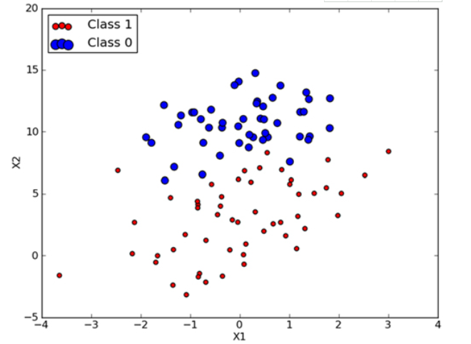
Save the data in testSet.txt Notepad, as shown in the following figure: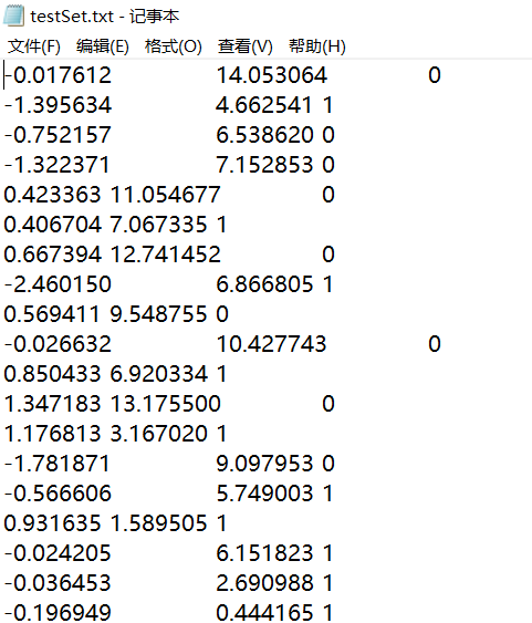
We can take these data as training samples of training model parameters. Seeing the training samples, we can intuitively understand the input of the algorithm and how we use these data to train the logistic regression classifier, and then use the trained model to predict new samples (test samples).

It can be seen that the data has two-dimensional characteristics, so the data can be displayed on a two-dimensional plane. We can take the first column of data as the value on the X1 axis and the second column of data as the value on the X2 axis. The last column of data is the classification label. These points are classified according to different labels.
Relevant codes:

#Open the text and read the data X1 and X2 of each line
def loadDataSet():
    dataMat = []      #Create data list
    labelMat = []      #Create label list
    fr = open('testSet.txt')    #Open file
    for line in fr.readlines():         #Read line by line
        lineArr = line.strip().split()       #Go to enter and put it in the list
        dataMat.append([1.0, float(lineArr[0]), float(lineArr[1])])    #Add data
        labelMat.append(int(lineArr[2]))      #Add label
    fr.close()    #Close file
    return dataMat, labelMat    
    
#sigmoid function
def sigmoid(inX):
    return 1.0/(1+exp(-inX))
    
#Gradient rise algorithm
dataMatrix = np.mat(dataMatIn)  # mat converted to numpy
    labelMat = np.mat(classLabels).transpose()  # Convert to numpy mat and transpose
    m, n = np.shape(dataMatrix)  # Returns the size of the dataMatrix. m is the number of rows and n is the number of columns.
    alpha = 0.001  # The moving step size, that is, the learning rate, controls the amplitude of the update.
    maxCycles = 500  # Maximum number of iterations
    weights = np.ones((n, 1))
    for k in range(maxCycles):
        h = sigmoid(dataMatrix * weights)  # Gradient rise vectorization formula
        error = labelMat - h
        weights = weights + alpha * dataMatrix.transpose() * error
    return weights.getA()  # Convert the matrix into an array and return the weight array

Test:

import logRegres
dataArr,labelMat=logRegres.loadDataSet()
print(logRegres.gradAscent(dataArr,labelMat))

result:

The regression coefficients of the three attributes are 4.12414349, 0.48007329 and -0.6168482 respectively

Analyze data: draw decision boundaries

Through the above experiments, a set of regression coefficients of the data are obtained. In short, the separation line between different types of data is determined. How to draw a separation line is described below.
Draw the function of the best fitting line between the data set and Logistic regression:

def plotBestFit(wei):
    import matplotlib.pyplot as plt
    weights = wei.getA()
    dataMat,labelMat=loadDataSet()
    dataArr = array(dataMat)
    n = shape(dataArr)[0] 
    xcord1 = []; ycord1 = []
    xcord2 = []; ycord2 = []
    for i in range(n):
        if int(labelMat[i])== 1:
            xcord1.append(dataArr[i,1]); ycord1.append(dataArr[i,2])
        else:
            xcord2.append(dataArr[i,1]); ycord2.append(dataArr[i,2])
    fig = plt.figure()
    ax = fig.add_subplot(111)
    ax.scatter(xcord1, ycord1, s=30, c='red', marker='s')
    ax.scatter(xcord2, ycord2, s=30, c='green')
    x = arange(-3.0, 3.0, 0.1)
    y = (-weights[0]-weights[1]*x)/weights[2]
    ax.plot(x, y)
    plt.xlabel('X1'); plt.ylabel('X2');
    plt.show()

Test:

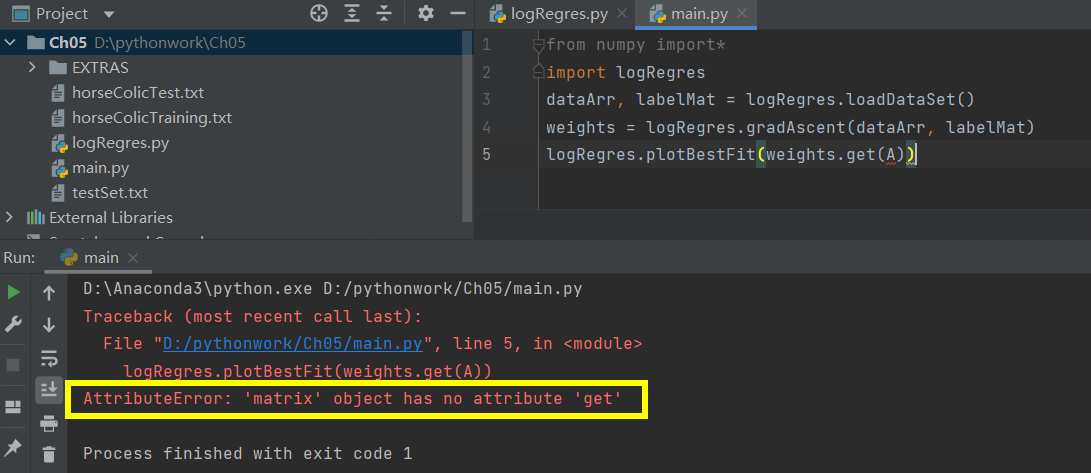
If you test according to the above figure, an error will be reported because of the version problem. Solution: delete getA().

from numpy import*
import logRegres
dataArr, labelMat = logRegres.loadDataSet()
weights = logRegres.gradAscent(dataArr, labelMat)
logRegres.plotBestFit(weights)

The output results are shown in the figure below:

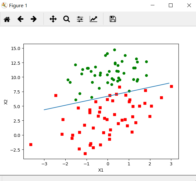
According to the figure, there are only two to four wrong points. However, the gradient rise algorithm has to traverse the whole data set every time it updates the regression coefficient. When there are thousands of samples, the computational complexity of the method is too high.

Training algorithm: random gradient rise

Methods: only one sample point at a time is used to update the regression coefficient, and the code is as follows:

def stocGradAscent0(dataMatrix, classLabels):
    m,n = shape(dataMatrix)
    alpha = 0.01
    weights = ones(n)   #initialize to all ones
    for i in range(m):
        h = sigmoid(sum(dataMatrix[i]*weights))
        error = classLabels[i] - h
        weights = weights + alpha * error * dataMatrix[i]
    return weights

Random gradient rise algorithm and gradient rise algorithm are very similar in code, but there are differences:
1. Both variable h and error are vectors, and the former is numeric
2. The former has no matrix conversion process, and the data types of all variables are Numpy arrays
Test:

from numpy import*
import logRegres
dataArr, labelMat = logRegres.loadDataSet()
weights = logRegres.stocGradAscent0(array(dataArr), labelMat)
logRegres.plotBestFit(weights)

The results are shown in the figure below:

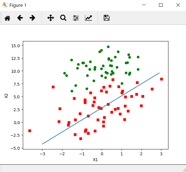
It can be seen that the effect is not as perfect as the previous regression gradient rise algorithm, and nearly one third of the samples are misclassified.

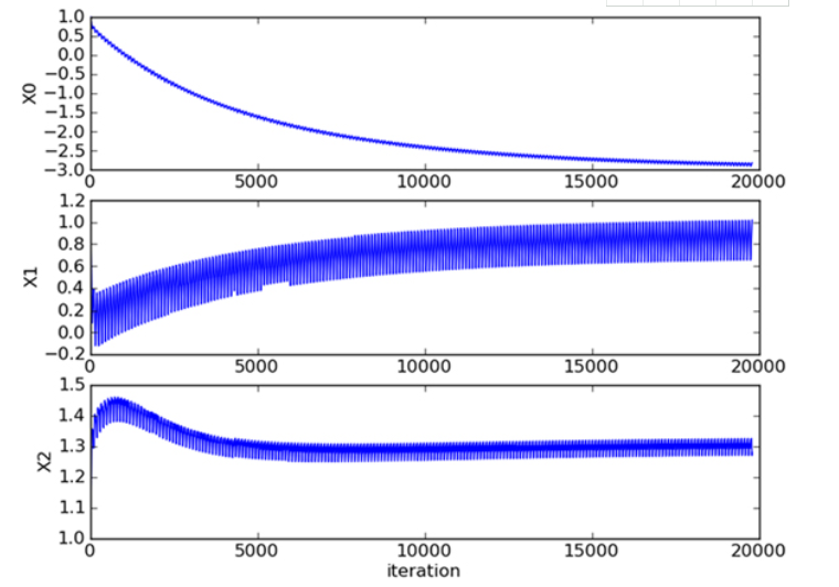
The following figure shows the relationship between the regression coefficient and the number of iterations in one traversal of the data set by running the random gradient rise algorithm. The regression coefficient can reach a stable value after a large number of iterations, and there are still local fluctuations.

Improved random gradient rise algorithm

Compared with the random gradient rise algorithm, two codes are added to improve it. The code is as follows:

def stocGradAscent1(dataMatrix, classLabels, numIter=150):
    m,n = np.shape(dataMatrix)                                                #Returns the size of the dataMatrix. m is the number of rows and n is the number of columns.
    weights = np.ones(n)                                                       #Parameter initialization
    for j in range(numIter):                                           
        dataIndex = list(range(m))
        for i in range(m):           
            alpha = 4/(1.0+j+i)+0.01                                            #Reduce the size of alpha by 1/(j+i) each time.
            randIndex = int(random.uniform(0,len(dataIndex)))                #Randomly selected samples
            h = sigmoid(sum(dataMatrix[randIndex]*weights))                    #Select a randomly selected sample and calculate h
            error = classLabels[randIndex] - h                                 #calculation error
            weights = weights + alpha * error * dataMatrix[randIndex]       #Update regression coefficient
            del(dataIndex[randIndex])                                         #Delete used samples
    return weights                           

The first improvement of the algorithm is that the alpha will be adjusted at each iteration, and although the alpha will decrease with the number of iterations, it will never decrease to 0, because there is still a constant term. The reason for this is to ensure that the new data still has an impact after multiple iterations. If the problem to be dealt with is dynamic, the above constant term can be appropriately increased to ensure that the new value can obtain a larger regression coefficient. Another point worth noting is that in the function of reducing alpha, alpha is reduced by 1/(j+i) each time, where j is the number of iterations and i is the subscript of the sample point. The second improvement is that only one sample point is used when tracking the new regression coefficient (optimal parameter), and the selected sample points are random, and the used sample points are not used in each iteration. This method effectively reduces the amount of calculation and ensures the regression effect.

The test results are as follows:

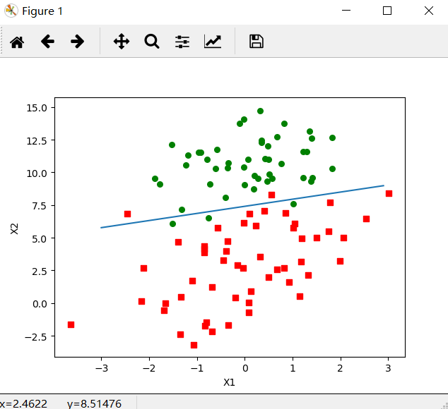
This time, only 150 times of traversal was done to the data, while the previous method was 500 times of traversal. This split line has the same effect as gradAscent(), but it requires less computation.

The improved random gradient rise algorithm has no periodic fluctuation and converges faster. It can be seen from the relationship between the regression coefficient and the number of iterations below: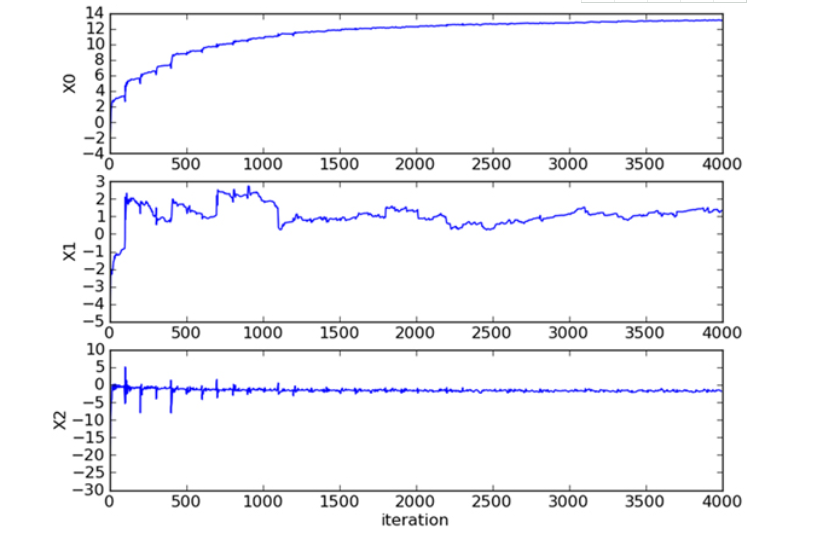

Data mining method for predicting forest fire using meteorological data by Logistic regression

Data preparation

1. Data source:
http://archive.ics.uci.edu/ml/datasets.php?format=&task=reg&att=&area=&numAtt=&numIns=100to1000&type=&sort=nameUp&view=table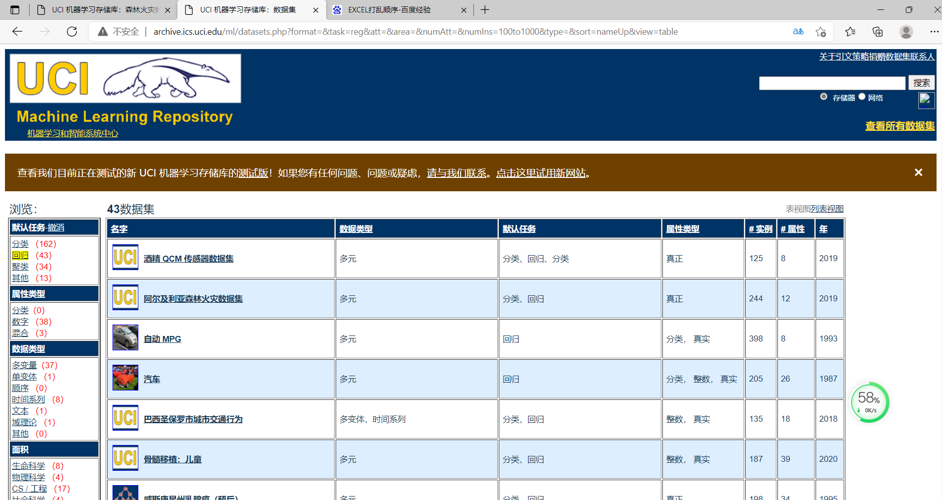

A total of 517 forest fires were selected, and the data dimension was 13, which met the experimental requirements.
Using python to disrupt 517 samples, 150 of them are taken as the test set, and the rest is the training set.

2. Data properties
Save the data download in the firetraining.txt file:

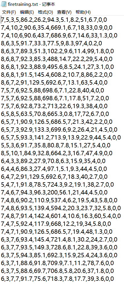
The 1st to 13th attributes respectively represent:
1. Spatial coordinates of the X - x axis in the map of montesinoo Park: 1 to 9
2. Spatial coordinates of Y - y axis in montesinoo Park Map: 2 to 9
3. Months of the year: 1 to 12
4. One day of the week: 1 to 7
5. FFMC - FFMC index of FWI system: 18.7 to 96.20
6. DMC - DMC index of FWI system: 1.1 to 291.3
7. DC DC index of FWI system: 7.9 to 860.6
8. ISI - ISI index of FWI system: 0.0 to 56.10
9. Temperature - temperature in degrees Celsius: 2.2 to 33.30
10.RH - relative humidity at%: 15.0 to 100
11. Wind speed - wind speed km / h: 0.40 to 9.40
12. Rain - outside rain mm / m2: 0.0 to 6.4
13. Area - burning area of forest (in hectares): 0.00 to 1090.84 (this output variable is very biased towards 0.0, so it may be meaningful to model with logarithmic transformation).

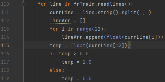
The 13th area - forest burning area, when it is 0.00, it means that there is no fire. When the burning area is > 0, we default to fire, that is, we read the last attribute of each line to judge whether there is a fire, as shown in the following code:

Regression classification function

1. Calculate the Sigmoid value

Take the regression coefficient and eigenvector as inputs to calculate the corresponding Sigmoid value. If the Sigmoid value is greater than 0.5, the function returns 1, otherwise it returns 0.

def classifyVector(inX, weights):
    prob = sigmoid(sum(inX * weights))
    if prob == 0.5:
        return 1.0
    else:
        return 0.0

2. Reading data from a text file

Read the data from "firetraining.txt" and put it in the data set. Additionally, process the last attribute of each row of data (the forest burning area is 0.00 to 1090.84, and convert those greater than 0 into 1, which is consistent with the binary output classifier). The training set data set tested reads all the data.

frTrain = open('firetraining.txt');
    trainingSet = [];
    trainingLabels = []
    for line in frTrain.readlines():
        currLine = line.strip().split(',')
        lineArr = []
        for i in range(12):
            lineArr.append(float(currLine[i]))
        temp = float(currLine[12]);
        if temp > 0.0:
            temp = 1.0
        else:
            temp = 0.0
        lineArr.append(temp)
        trainingSet.append(lineArr)

3. Scramble data

Why bother? Because the data of the initial data set is located in the front and the last column is basically 0 (the combustion area is 0, i.e. there is no fire), it does not show a sense of clutter until the end. In order to reduce accidental errors, the data is disturbed:

random.shuffle(trainingSet)

4. Generate test set and training set

    trainingSet = array(trainingSet)
    trainingLabels = trainingSet[:, -1] #Take the last attribute of each sample
    trainingSet = trainingSet[:,:-1] #Take all attributes of each sample except the last attribute
    testSet = trainingSet[:150] #Take the first 150 as the test set and generate the test set
    testLabel = trainingLabels[:150] #Take the first 150 as test set labels
    trainingSet = trainingSet[150:] #Generate training set
    trainingLabels= trainingLabels[150:]
    print(trainingLabels.shape, trainingSet.shape)
    print(testLabel.shape, testSet.shape)

Output results:

5. Calculate the regression coefficient vector

Here, the number of iterations can be set freely:

 trainWeights = stocGradAscent1(array(trainingSet), trainingLabels, 500)
    errorCount = 0;
    for i in range(len(testSet)):
        if int(classifyVector(testSet[i], trainWeights)) != testLabel[i]:
                errorCount += 1
    errorRate = (float(errorCount) / 150)
    print("the error rate of this test is: %f" % errorRate)
    return errorRate

6. Test

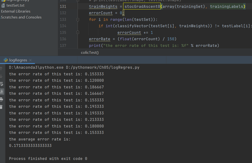
1. When using the original random gradient algorithm on the training set:

2. When using the improved random gradient algorithm on the training set:

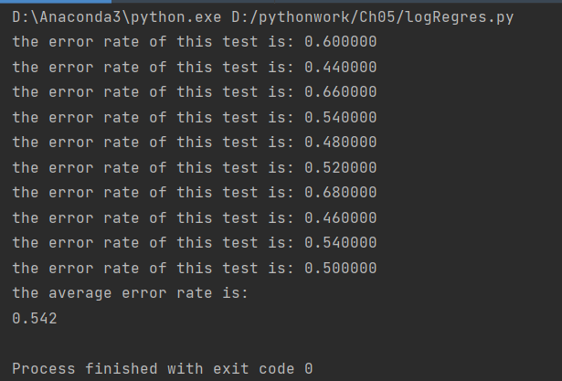
2.1 When using 100 iterations on the training set:

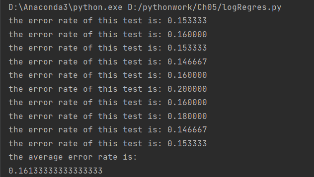
2.2 when 500 iterations are used on the training set:

Summary

1. Comparison of 2.1 and 2.2: the training set uses 500 iterations, and the experimental result is that the error rate of 2.2 is significantly reduced, indicating that the effect of 500 iterations is better than 100 iterations, and the number of iterations cannot be less.
2. Compared with 1 and 2, although the error rate of the improved random gradient algorithm is lower, the running time is longer and the running speed is slower, while the error rate of the original random gradient algorithm is higher than that of the improved algorithm, but the running time is shorter. Therefore, when there is less data in the data set, the original random gradient algorithm can be used. When there are many data, the improved random gradient algorithm is used to solve it.

Experimental summary

In this experiment, with the help of course ppt and machine learning materials, as well as reading a large number of blogs on csdn, I learned logical regression, mastered linear regression and analyzed data, so as to make the data conform to the input of decision tree algorithm. However, when compiling data, using UCI machine learning database leads to ideal experimental results, which is much better than the data compiled by the decision tree last time.