So Bayesian statistical analysis is so simple? Learn about this technique (live data sharing)~~

Posted by kornlord283 on Tue, 23 Nov 2021 16:31:13 +0100

Today, I will introduce you a very useful statistical analysis skill - r-bayestr. Unlike most other R packages, which only provide a limited set of indexes (such as point estimation and CI), this package can provide a comprehensive and consistent set of functions to analyze and describe the posterior distribution generated by various model objects, including popular modeling packages, such as rstanarm, brms or BayesFactor. For more information about the package, please refer to the R-bayestestR official website [1]

The following is a brief introduction to the usage of this package, mainly as follows:

Features

In the Bayesian framework, parameters are estimated as distributions in a probabilistic manner. These distributions can be summarized and described by the following four indexes. For more other features, please refer to: Many other Features[2]

Centrality
- mean(),median(),map_estimate() is used to estimate the pattern.
- point_estimate() can be used to get them immediately and run them directly on the model.
Uncertainty
- hdi() represents the highest density interval (HDI) or eti() represents the equal tail interval (ETI).
- ci() can be used as a general method of confidence interval (CI).
Effect Existence: whether the effect is different from 0.
- p_direction() represents the Bayesian equivalent of the p value of the frequency school.
- p_pointnull() indicates the probability of the null hypothesis (h0 = 0) compared to the most likely hypothesis (MAP).
- bf_pointnull() is used for classical Bayesian factor (BF) to evaluate the possibility of the existence and absence of effects (h0 = 0).
Effect Significance: whether the effect size can be considered as non negligible.
- p_ The probability that the rope () effect falls within the actual equivalent area (ROPE).
- bf_rope() calculates the Bayesian factor based on the null value defined by the region (ROPE).
- p_significance() combines the equivalent region with the directional probability.

Description of r-bayestr package_ Some features can be calculated by posterior (), as follows:

library(bayestestR)
bayestestR::describe_posterior(
  rnorm(10000),
  centrality = "median",
  test = c("p_direction", "p_significance")
)

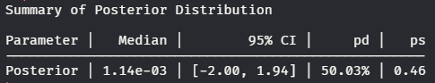
Example Of describe_posterior()

More about describe_ For an introduction to posterior(), refer to: describe_ Introduction to posterior() function [3]

Point-estimates

As one of the most commonly used bayestr packet distribution features, point estimates () can calculate various point estimates (such as mean, median or MAP) to describe the posterior distribution as follows:

posterior <- distribution_gamma(10000, 1.5)  # Generate a skewed distribution
centrality <- point_estimate(posterior)  # Get indices of centrality
plot(centrality) +
  labs(
       title = "Example of <span style='color:#D20F26'>bayestestR::point_estimate function</span>",
       subtitle = "processed charts with <span style='color:#1A73E8'>point_estimate()</span>",
       caption = "Visualization by <span style='color:#0057FF'>DataCharm</span>") +
  hrbrthemes::theme_ipsum(base_family = "Roboto Condensed") +
  theme(
    plot.title = element_markdown(hjust = 0.5,vjust = .5,color = "black",
                                  size = 20, margin = margin(t = 1, b = 12)),
    plot.subtitle = element_markdown(hjust = 0,vjust = .5,size=15),
    plot.caption = element_markdown(face = 'bold',size = 12))

Example Of point_estimate()

Uncertainty (CI)

hdi() calculates the highest density interval (HDI) of a posteriori distribution, that is, the interval containing all points in the interval has a higher probability density than the points outside the interval. HDI can be used in the context of Bayesian posteriori representation of confidence interval (CI).

Unlike the 2.5% equal tailed interval usually excluded from each tail of the distribution, HDI is not an equal tailed interval, so it always includes the mode of a posteriori distribution.

By default, hdi() returns the interval of 89% (ci = 0.89), and the interval of 95% is more stable. The visual display is as follows:

「Highest Density Interval (HDI)」:

m <<- stan_glm(Sepal.Length ~ Petal.Width * Species, data = iris, refresh = 0)
result <- hdi(m,ci = .89)

plot(result) +
  labs(
    title = "Example of <span style='color:#D20F26'>bayestestR::hdi function</span>",
    subtitle = "processed charts with <span style='color:#1A73E8'>hdi(ci=.89)</span>",
    caption = "Visualization by <span style='color:#0057FF'>DataCharm</span>") +
  hrbrthemes::theme_ipsum(base_family = "Roboto Condensed") +
  theme(
    plot.title = element_markdown(hjust = 0.5,vjust = .5,color = "black",
                                  size = 20, margin = margin(t = 1, b = 12)),
    plot.subtitle = element_markdown(hjust = 0,vjust = .5,size=15),
    plot.caption = element_markdown(face = 'bold',size = 12))

Example Of hdi(ci=.89)

「Equal-Tailed Interval (ETI)」:

m2 <- eti(m,ci = .89)

plot(m2) +
  labs(
    title = "Example of <span style='color:#D20F26'>bayestestR::eti function</span>",
    subtitle = "processed charts with <span style='color:#1A73E8'>eti(ci=.89)</span>",
    caption = "Visualization by <span style='color:#0057FF'>DataCharm</span>") +
  hrbrthemes::theme_ipsum(base_family = "Roboto Condensed") +
  theme(
    plot.title = element_markdown(hjust = 0.5,vjust = .5,color = "black",
                                  size = 20, margin = margin(t = 1, b = 12)),
    plot.subtitle = element_markdown(hjust = 0,vjust = .5,size=15),
    plot.caption = element_markdown(face = 'bold',size = 12))

Example Of eti(ci=.89)

Existence and Significance Testing

「Probability of Direction (pd)」:

p_direction() calculates the probability of direction (PD, also known as maximum effect probability MPE). It varies from 50% to 100% (i.e. 0.5 and 1), which can be interpreted as the probability (expressed as a percentage) that the parameter (described by a posterior distribution) is strictly positive or negative, and this index is very similar to the p value (i.e. strong correlation).

posterior <- distribution_normal(10000, 0.4, 0.2)
m3 <- p_direction(posterior)
plot(m3) +
  scale_fill_manual(values = c("#E91E63","#FFC107"))+
  labs(
    title = "Example of <span style='color:#D20F26'>bayestestR::p_direction function</span>",
    subtitle = "processed charts with <span style='color:#1A73E8'>p_direction()</span>",
    caption = "Visualization by <span style='color:#0057FF'>DataCharm</span>") +
  hrbrthemes::theme_ipsum(base_family = "Roboto Condensed") +
  theme(
    plot.title = element_markdown(hjust = 0.5,vjust = .5,color = "black",
                                  size = 20, margin = margin(t = 1, b = 12)),
    plot.subtitle = element_markdown(hjust = 0,vjust = .5,size=15),
    plot.caption = element_markdown(face = 'bold',size = 12))

Example Of p_direction

ROPE

rope() calculates the percentage of a posteriori distributed HDI(89% HDI by default) located in the actual equivalent region.

posterior <- distribution_normal(10000, 0.4, 0.2)
m4 <- rope(posterior, range = c(-0.1, 0.1),)
plot(m4) +
  scale_fill_manual(values = c("#E91E63","#FFC107"))+
  labs(
    title = "Example of <span style='color:#D20F26'>bayestestR::rope function</span>",
    subtitle = "processed charts with <span style='color:#1A73E8'>rope()</span>",
    caption = "Visualization by <span style='color:#0057FF'>DataCharm</span>") +
  hrbrthemes::theme_ipsum(base_family = "Roboto Condensed") +
  theme(
    plot.title = element_markdown(hjust = 0.5,vjust = .5,color = "black",
                                  size = 20, margin = margin(t = 1, b = 12)),
    plot.subtitle = element_markdown(hjust = 0,vjust = .5,size=15),
    plot.caption = element_markdown(face = 'bold',size = 12))

Example Of ROPE()

Bayes Factor

bayesfactor_parameters() calculates a Bayesian factor for null values (points or intervals) based on a priori and a posteriori samples of a single parameter. This Bayesian factor represents the extent to which the quality of a posteriori distribution is far from or close to null values (relative to a priori distribution), indicating whether null values become smaller or more likely to give observed data.

##  Bayes Factor
prior <- distribution_normal(10000, mean = 0, sd = 1)
posterior <- distribution_normal(10000, mean = 1, sd = 0.7)

m5 <- bayesfactor_parameters(posterior, prior, direction = "two-sided", null = 0)
m5

plot(m5)+
  scale_fill_material_d(palette = "ice") +
  scale_color_material_d(palette = "ice") +
  labs(
    title = "Example of <span style='color:#D20F26'>bayestestR::bayesfactor_parameters function</span>",
    subtitle = "processed charts with <span style='color:#1A73E8'>bayesfactor_parameters()</span>",
    caption = "Visualization by <span style='color:#0057FF'>DataCharm</span>") +
  hrbrthemes::theme_ipsum(base_family = "Roboto Condensed") +
  theme(
    plot.title = element_markdown(hjust = 0.5,vjust = .5,color = "black",
                                  size = 20, margin = margin(t = 1, b = 12)),
    plot.subtitle = element_markdown(hjust = 0,vjust = .5,size=15),
    plot.caption = element_markdown(face = 'bold',size = 12))

Example Of bayesfactor_parameters

For more details on bayesfactor_parameters(), please refer to bayesfactor_parameters()[4]

summary

Today's tweet briefly introduces the commonly used Bayesian principle r-baytestr in Statistics (it may involve less professional aspects, but the original intention is to understand this skill). It can not only calculate various indicators, but also use appropriate visual charts. I hope you can learn more about this useful statistical analysis package.

reference material

[1]

R-bayestr official website: https://easystats.github.io/bayestestR/index.html .

[2]

Bayestestr other features: https://easystats.github.io/bayestestR/reference/index.html .

[3]

Description_posterior() function: https://easystats.github.io/bayestestR/reference/describe_posterior.html .

[4]

bayesfactor_parameters() introduction: https://easystats.github.io/bayestestR/reference/bayesfactor_parameters.html .

Just order one if you like 👇

Programmer Think