The data set is referred to the following website:

House Prices - Advanced Regression Techniques | KagglePredict sales prices and practice feature engineering, RFs, and gradient boostinghttps://www.kaggle.com/c/house-prices-advanced-regression-techniques

preface:

This paper is divided into two periods, which is too long and inconvenient. This paper mainly introduces the data analysis steps of the data set, including data preprocessing, data mining, selecting appropriate model algorithms to solve problems. The ability is limited for reference only. The features are explained in English. If necessary, you can refer to the following:

  SalePrice: the sales price of the real estate, which is denominated in US dollars. Target variable to be predicted
-MSSubClass: Identifies the type of dwelling involved in the sale
-MSZoning: The general zoning classification
-Lotfront: linear feed of street connected to property
-LotArea: Lot size in square feet
-Street: Type of road access
-Alley: Type of alley access
-LotShape: General shape of property
-LandContour: Flatness of the property
-Utilities: Type of utilities available
-LotConfig: Lot configuration configuration
-LandSlope: Slope of property
-Neighborhood: Physical locations within Ames city limits
-Condition1: Proximity to main road or railroad
-Condition2: Proximity to main road or railroad (if a second is present)
-BldgType: Type of dwelling
-HouseStyle: Style of dwelling
-Overall material and finish quality
-OverallCond: Overall condition rating
-Yearbuild: original construction date
-Yearremoddadd: Remodel date
-Roof style: type of roof
-Roof material: roof material
-Exterior 1st: exterior covering on house facade materials
-Exterior 2nd: exterior covering on house (if more than one material)
-MasVnrType: Masonry veneer type decorative stone type
-MasVnrArea: Masonry veneer area in square feet
-Exterior material quality
-ExterCond: Present condition of the material on the exterior
-Foundation: Type of foundation
-BsmtQual: Height of the basement
-BsmtCond: General condition of the basement
-Bsmtexposure: walk out or garden level basement walls
-BsmtFinType1: Quality of basement finished area
-Bsmtfinsf1: type 1 finished square feet
-BsmtFinType2: Quality of second finished area (if present)
-Bsmtfinsf2: type 2 finished square feet
-Bsmtunfsf: unfinished square fee of basement area
-TotalBsmtSF: Total square feet of basement area
-Heating: Type of heating
-Heating quality and condition
-Central air: central air conditioning
-Electrical: Electrical system
-1stFlrSF: First Floor square feet
-2ndFlrSF: Second floor square feet
-LowQualFinSF: Low quality finished square feet (all floors)
-GrLivArea: Above grade (ground) living area square feet
-Bsmtfullbath: number of basement full bathrooms
-Bsmthalfbath: number of half bathrooms in basement half bathrooms
-FullBath: Full bathrooms above grade
-HalfBath: Half baths above grade
-Bedroom: Number of bedrooms above basement level
-KitchenAbvGr: Number of kitchens
-Kitchen quality
-TotRmsAbvGrd: Total rooms above grade (does not include bathrooms)
-Functional: Home functional rating
-Fireplaces: Number of fireplaces
-Fireplace Qu: Fireplace quality
-Garage type: garage location
-Garage yrblt: year garage was built
-Garage finish: interior finish of the garage
-Garage cars: size of garage in car capacity
-Garage area: size of garage in square feet
-Garage quality
-Garage condition: garage condition
-Pavedderive: paved driveway
-Wooddeck SF: wood deck area in square feet
-OpenPorchSF: Open porch area in square feet
-Enclosed porch: enclosed porch area in square feed
-3ssnporch: three search porch area in square feet
-Screen porch: screen porch area in square feet
-Pool area: pool area in square feet
-PoolQC: Pool quality
-Fence: Fence quality
-MiscFeature: Miscellaneous feature not covered in other categories
-MiscVal: $Value of miscellaneous feature
-MoSold: Month Sold
-YrSold: Year Sold
-SaleType: Type of sale
-SaleCondition: Condition of sale  

  First, import the required packages:

import numpy as np 
import pandas as pd 
from sklearn.preprocessing import OrdinalEncoder
from sklearn.preprocessing import StandardScaler
from sklearn.preprocessing import MinMaxScaler
import seaborn as sns
from sklearn.model_selection import train_test_split
from tensorflow import keras
from tensorflow.keras import layers
from tensorflow.keras.models import Sequential
from tensorflow.keras.layers import Dense, Activation
from tensorflow.keras.optimizers import Adam

Import data:

df_train = pd.read_csv('C:/Users/Desktop/Big data exercise/House price forecast/train.csv')
df_test = pd.read_csv('C:/Users/Desktop/Big data exercise/House price forecast/test.csv')

First, let's take a look at the overview of the training set:

train_data.describe()

train_data.info()

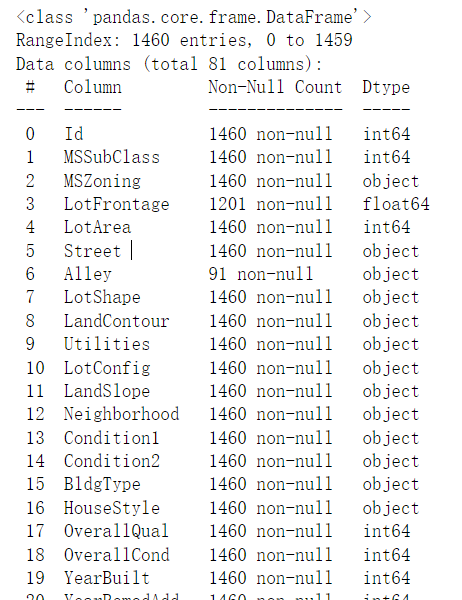
  There are many null values. It seems that null values need to be processed below, otherwise the accuracy of the result is very poor.

Next, I want to see the distribution of this price

sns.distplot(train_data['SalePrice']);

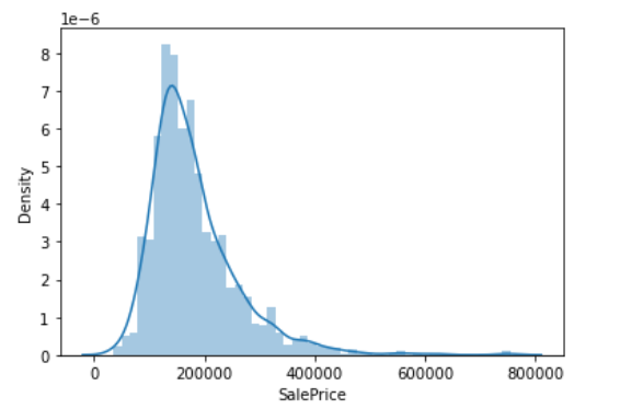
  The price distribution is pretty good, a little biased.

Next, we will process the vacancy value and calculate the vacancy value:

total = train_data.isnull().sum().sort_values(ascending=False)
percent = (train_data.isnull().sum()/train_data.isnull().count()).sort_values(ascending=False)
missing_data = pd.concat([total, percent], axis=1, keys=['Total', 'Percent'])
missing_data.head(20)

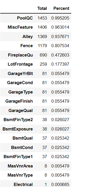
Start deleting and populating null values

#Delete features that have no value
train_data['LotFrontage'].fillna((train_data['LotFrontage'].mean()), inplace=True)
train_data.drop('Alley', axis=1, inplace=True)
train_data.drop('PoolQC', axis=1, inplace=True)
train_data.drop('Fence', axis=1, inplace=True)
train_data.drop('MiscFeature', axis=1, inplace=True)

 

#Populate data

train_data['MasVnrType'].fillna((train_data['MasVnrType'].value_counts().index[0]), inplace=True)
train_data['MasVnrArea'].fillna((train_data['MasVnrArea'].mean()), inplace=True)
train_data['BsmtQual'].fillna((train_data['BsmtQual'].value_counts().index[0]), inplace=True)
train_data['BsmtCond'].fillna((train_data['BsmtCond'].value_counts().index[0]), inplace=True)
train_data['BsmtExposure'].fillna((train_data['BsmtExposure'].value_counts().index[0]), inplace=True)
train_data['BsmtFinType1'].fillna((train_data['BsmtFinType1'].value_counts().index[0]), inplace=True)
train_data['BsmtFinType2'].fillna((train_data['BsmtFinType2'].value_counts().index[0]), inplace=True)
train_data['Electrical'].fillna((train_data['Electrical'].value_counts().index[0]), inplace=True)
train_data.drop('FireplaceQu', axis=1, inplace=True)
train_data['GarageType'].fillna((train_data['GarageType'].value_counts().index[0]), inplace=True)
train_data['GarageYrBlt'].fillna((train_data['GarageYrBlt'].mean()), inplace=True)
train_data['GarageFinish'].fillna((train_data['GarageFinish'].value_counts().index[0]), inplace=True)
train_data['GarageQual'].fillna((train_data['GarageQual'].value_counts().index[0]), inplace=True)
train_data['GarageCond'].fillna((train_data['GarageCond'].value_counts().index[0]), inplace=True)

Extract important indicators for processing:

cols = [
    'MSZoning', 'Street', 'LotShape', 'LandContour', 'Utilities', 'LotConfig', 
    'LandSlope', 'Neighborhood', 'Condition1', 'Condition2', 'BldgType', 'HouseStyle',
    'RoofStyle', 'RoofMatl', 'Exterior1st', 'Exterior2nd', 'MasVnrType', 'ExterQual', 
    'ExterCond', 'Foundation', 'BsmtQual', 'BsmtCond', 'BsmtExposure', 'BsmtFinType1',
        'BsmtFinType2', 'Heating', 'HeatingQC', 'CentralAir', 'Electrical', 'KitchenQual',
    'Functional', 'GarageType', 'GarageFinish', 'GarageQual', 'GarageCond', 'PavedDrive',
    'SaleType', 'SaleCondition']

train_data[cols] = train_data[cols].astype('category')

We encode the columns:

class sklearn.preprocessing.OrdinalEncoder

(*, categories='auto', dtype=<class 'numpy.float64'>)

Encode the classification features into an integer array. The input to the converter should be an array of integers or strings representing the values used for classification (discrete) features. The feature is converted to an ordinal integer. This results in a column of integers (0 to n_categories-1) for each feature.

fit(X[， y])	Fit the ordinal encoder to X.
fit_transform(X[， y])	Adapt the data and then transform it.
get_params([deep])	Gets the parameters for this estimator.
inverse_transform(X)	Converts data back to its original representation.
set_params (* * parameter)	Set parameters for this estimator.
transform(X)	Convert X to serial number code.

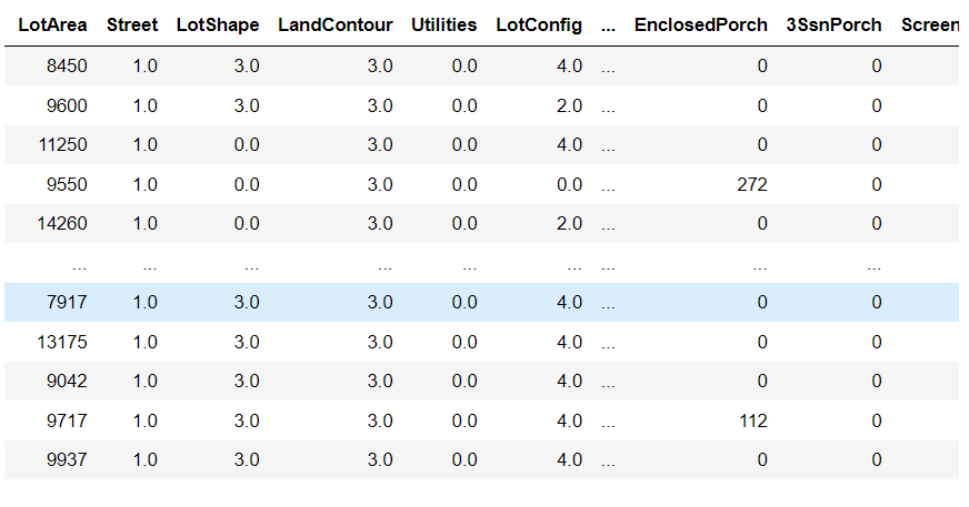
Let it generate codes, so that we can observe our data more intuitively:

encoder = OrdinalEncoder()
encoder.fit(train_data[cols])
train_data[cols] = encoder.transform(train_data[cols])
train_data

  Start correlation analysis:

# Looking for relevance
corr_matrix = train_data.corr()#Pearson correlation coefficient
corr_values = corr_matrix["SalePrice"].sort_values(ascending=False)
top_10 = corr_values[:10]
bottom_10 = corr_values[-10:]

 

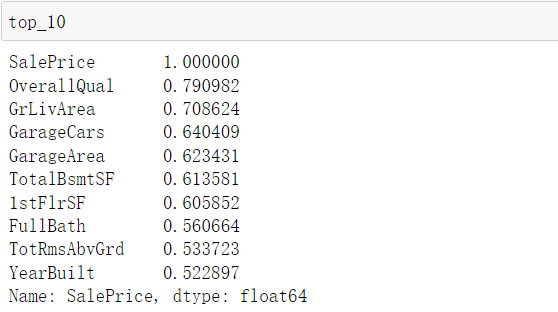
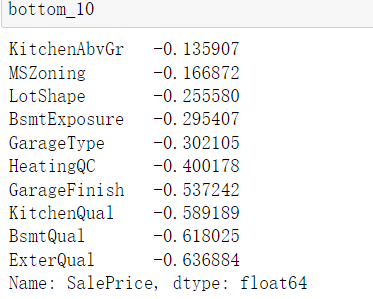
  Select the best column according to the above;

# Select the best column according to the above

best_cols = [
    'OverallQual', 'GrLivArea', 'GarageCars', 'GarageArea', 'TotalBsmtSF', '1stFlrSF',
    'GarageFinish', 'KitchenQual', 'BsmtQual', 'ExterQual', 'SalePrice'
]

train_data = train_data[best_cols]

We use   three σ Data cleaning in principle:

Based on the equal precision repeated measurement of normal distribution, the interference or noise of singular data is difficult to meet the normal distribution.

If the absolute value of the residual error of a certain measurement value in a set of measurement data ν i>3 σ， Then the measured value is bad and should be eliminated. Usually equal to ± 3 σ The error of is taken as the limit error, and for the random error of normal distribution, it falls within ± 3 σ The probability is only 0.27%, which is very unlikely to occur in a limited number of measurements, so there are 3 σ Guidelines. three σ The criterion is the most commonly used and simplest criterion for judging gross error. It is generally used when the number of measurements is sufficient (n ≥ 30) or when n > 10 makes rough judgment.

#Delete outliers use quartiles to improve the deletion of data that may change the result
train_data = train_data[train_data['GrLivArea'] <= train_data['GrLivArea'].quantile(0.75)]
train_data = train_data[train_data['GarageArea'] <= train_data['GarageArea'].quantile(0.75)]
train_data = train_data[train_data['TotalBsmtSF'] <= train_data['TotalBsmtSF'].quantile(0.75)]
train_data = train_data[train_data['1stFlrSF'] <= train_data['1stFlrSF'].quantile(0.75)]

For data normalization processing, please refer to (63 messages) data processing - scipy.stats.norm function, the role of normalization_ am_student blog - CSDN blog:  

cols = ['GrLivArea', 'GarageArea', 'TotalBsmtSF', '1stFlrSF']
standard_scaler = StandardScaler()
train_data[cols] = standard_scaler.fit_transform(train_data[cols])

At this time, let's see what kind of state our data is:  

train_data.describe()

X = train_data.drop('SalePrice',axis=1).values
y = train_data['SalePrice'].values

Separate data in training set and test set:

X_train, X_test, y_train, y_test = train_test_split(X, y, test_size=0.3, random_state=42)

  Check the data of training data and test data:

print("X_train - ",X_train.shape)
print("y_train - ",y_train.shape)
print("X_test - ",X_test.shape)
print("y_test - ",y_test.shape)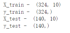

Data standardization:

scaler = MinMaxScaler()
X_train= scaler.fit_transform(X_train)
X_test = scaler.transform(X_test)

  Due to the space problem, the model will be listed in the following, which is under urgent completion

At the same time, we can pay attention to the dynamic trend in official account and discuss together.