In recent days, I have studied sorting algorithm and read many blogs. I found that some articles on the Internet do not explain sorting algorithm thoroughly, and many codes are wrong. For example, some articles directly use the Collection.sort() function to sort each bucket in the "bucket sorting" algorithm, which can achieve results, But it is impossible for algorithm research. Therefore, according to the articles I read these days, I have sorted out a relatively complete summary of sorting algorithms. All algorithms in this paper are implemented in JAVA and issued after my debugging. If there are errors, please point out them.

0. Description of sorting algorithm

0.1 definition of sorting

Sort a sequence of objects according to a keyword.

0.2 description of terms

• Stable: if a is in front of b and a=b, a is still in front of b after sorting;
• Unstable: if a was originally in front of b and a=b, a may appear after b after sorting;
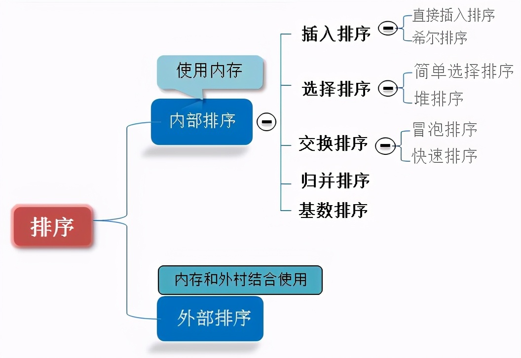
• Internal sorting: all sorting operations are completed in memory;
• External sorting: because the data is too large, the data is placed on the disk, and the sorting can only be carried out through the data transmission of disk and memory;
• Time complexity:   The time spent executing an algorithm.
• Space complexity: the amount of memory required to run a program.

0.3 algorithm summary

Explanation of picture terms:

• n: Data scale
• k: Number of "barrels"
• In place: constant memory, no additional memory
• Out place: taking up extra memory

0.5 algorithm classification

0.6 difference between comparison and non comparison

Common quick sort, merge sort, heap sort and bubble sort belong to comparative sort. In the final result of sorting, the order between elements depends on the comparison between them. Each number must be compared with other numbers to determine its position.
In bubble sort, the problem scale is n, and because it needs to be compared n times, the average time complexity is O(n) ²). In sorting such as merge sort and quick sort, the problem scale is reduced to logN times by divide and conquer, so the time complexity is O(nlogn) on average.
The advantage of comparative sorting is that it is suitable for data of all sizes and does not care about the distribution of data. It can be said that comparative sorting is suitable for all situations that need sorting.

Count sort, cardinality sort and bucket sort belong to non comparison sort. Non comparison sort is to sort by determining how many elements should be before each element. For array arr, calculating how many elements are before arr[i] uniquely determines the position of arr[i] in the sorted array.
Non comparative sorting can be solved by determining the number of existing elements before each element, and all traversals can be solved at one time. The time complexity of the algorithm is O(n).
The time complexity of non comparative sorting is low, but because non comparative sorting needs to occupy space to determine the unique location, it has certain requirements for data scale and data distribution.

1. Bubble Sort

Bubble sorting is a simple sorting algorithm. It repeatedly visits the sequence to be sorted, compares two elements at a time, and exchanges them if they are in the wrong order. The work of visiting the sequence is repeated until there is no need to exchange, that is, the sequence has been sorted. The name of this algorithm is because the smaller elements will be slower through exchange Slowly "float" to the top of the sequence.

1.1 algorithm description

• Compare adjacent elements. If the first is larger than the second, swap them two;
• Do the same for each pair of adjacent elements, from the first pair at the beginning to the last pair at the end, so that the last element should be the largest number;
• Repeat the above steps for all elements except the last one;
• Repeat steps 1 to 3 until the sorting is completed.

1.2 dynamic diagram demonstration

1.3 code implementation

 1  　　/**
 2      * Bubble sorting
 3      *
 4      * @param array
 5      * @return
 6      */
 7     public static int[] bubbleSort(int[] array) {
 8         if (array.length == 0)
 9             return array;
10         for (int i = 0; i < array.length; i++)
11             for (int j = 0; j < array.length - 1 - i; j++)
12                 if (array[j + 1] < array[j]) {
13                     int temp = array[j + 1];
14                     array[j + 1] = array[j];
15                     array[j] = temp;
16                 }
17         return array;
18     }

1.4 algorithm analysis

Best case: T(n) = O(n) worst case: T(n) = O(n2) average case: T(n) = O(n2)

2. Selection Sort

One of the most stable sorting algorithms, because no matter what data goes in, it is O(n2) time complexity, so when using it, the smaller the data size is, the better. The only advantage may be that it does not occupy additional memory space. Theoretically, selective sorting may also be the most common sorting method that ordinary people think of.

Selection sort is a simple and intuitive sorting algorithm. Its working principle: first find the smallest (large) element in the unordered sequence and store it at the beginning of the sorting sequence, then continue to find the smallest (large) element from the remaining unordered elements, and then put it at the end of the sorted sequence. And so on until all elements are sorted.

2.1 algorithm description

The direct selection sorting of n records can get ordered results after n-1 times of direct selection sorting. The specific algorithm is described as follows:

• Initial state: the disordered area is R[1..n], and the ordered area is empty;
• At the beginning of the i-th sequence (i=1,2,3... n-1), the current ordered area and unordered area are R[1..i-1] and R(i..n) respectively. This sequence selects the record R[k] with the smallest keyword from the current unordered area and exchanges it with the first record R in the unordered area, so that R[1..i] and R[i+1..n) become a new ordered area with an increase in the number of records and a new unordered area with a decrease in the number of records respectively;
• At the end of n-1 trip, the array is ordered.

2.2 dynamic diagram demonstration

　　

2.3 code implementation

　　/**
     * Select sort
     * @param array
     * @return
     */
    public static int[] selectionSort(int[] array) {
        if (array.length == 0)
            return array;
        for (int i = 0; i < array.length; i++) {
            int minIndex = i;
            for (int j = i; j < array.length; j++) {
                if (array[j] < array[minIndex]) //Minimum number found
                    minIndex = j; //Save the index of the smallest number
            }
            int temp = array[minIndex];
            array[minIndex] = array[i];
            array[i] = temp;
        }
        return array;
    }

2.4 algorithm analysis

Best case: T(n) = O(n2) worst case: T(n) = O(n2) average case: T(n) = O(n2)

3. Insertion Sort

The algorithm description of insertion sort is a simple and intuitive sorting algorithm. Its working principle is to construct an ordered sequence. For unordered data, scan from back to front in the sorted sequence, find the corresponding position and insert it. In the implementation of insertion sort, in place sort is usually adopted (i.e. sort that only needs the extra space of O(1)) Therefore, in the process of scanning from back to front, it is necessary to repeatedly move the sorted elements back step by step to provide insertion space for the latest elements.

3.1 algorithm description

Generally speaking, insertion sorting is implemented on the array using in place. The specific algorithm is described as follows:

• Starting from the first element, the element can be considered to have been sorted;
• Take out the next element and scan from back to front in the sorted element sequence;
• If the element (sorted) is larger than the new element, move the element to the next position;
• Repeat step 3 until the sorted element is found to be less than or equal to the position of the new element;
• After inserting the new element into this position;
• Repeat steps 2 to 5.

3.2 dynamic diagram demonstration

3.2 code implementation

　　/**
     * Insert sort
     * @param array
     * @return
     */
    public static int[] insertionSort(int[] array) {
        if (array.length == 0)
            return array;
        int current;
        for (int i = 0; i < array.length - 1; i++) {
            current = array[i + 1];
            int preIndex = i;
            while (preIndex >= 0 && current < array[preIndex]) {
                array[preIndex + 1] = array[preIndex];
                preIndex--;
            }
            array[preIndex + 1] = current;
        }
        return array;
    }

3.4 algorithm analysis

Best case: T(n) = O(n) worst case: T(n) = O(n2) average case: T(n) = O(n2)

4. Shell Sort

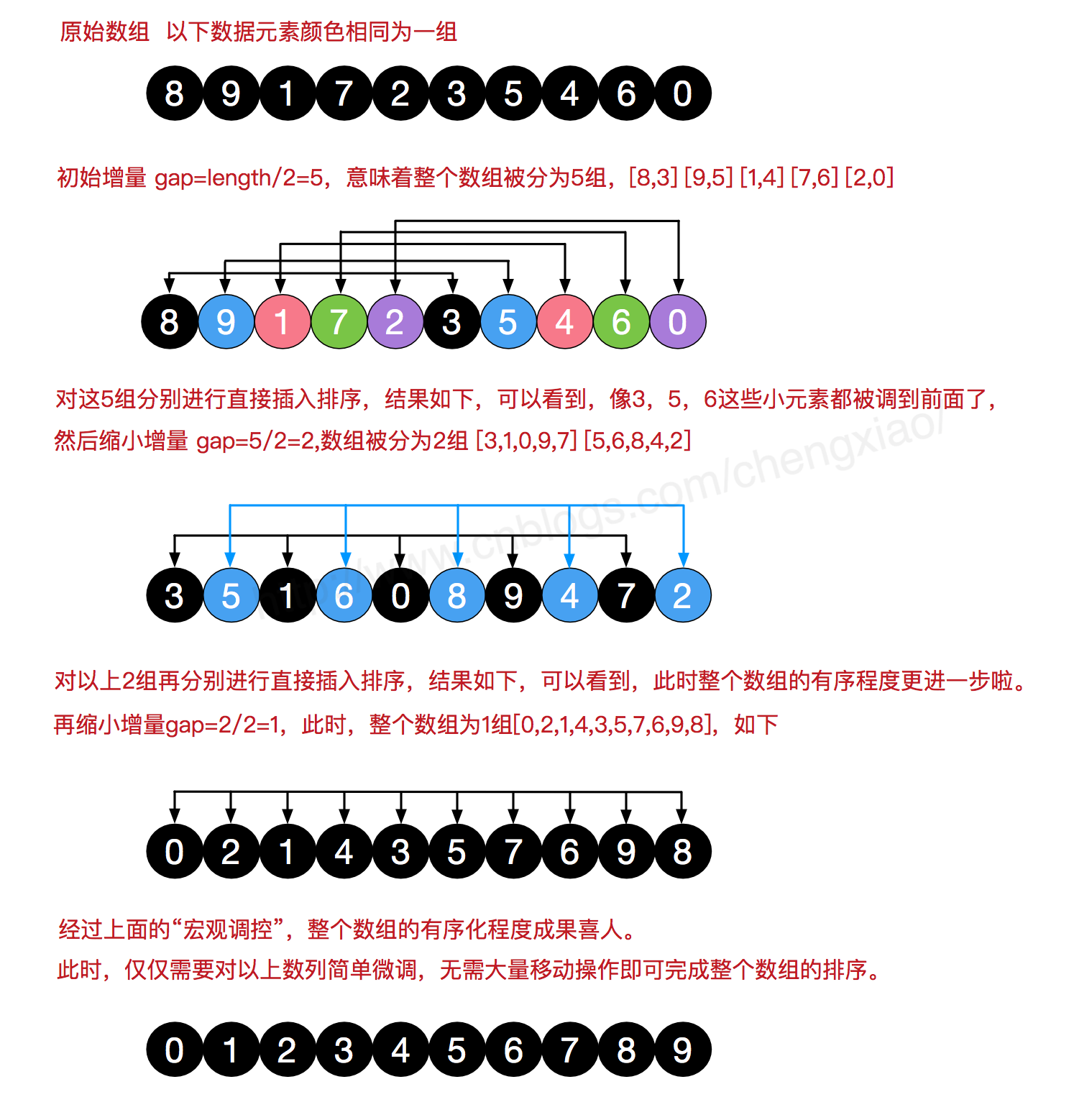
Hill sorting is a sort algorithm proposed by Donald Shell in 1959. Hill sort is also an insertion sort. It is a more efficient version of simple insertion sort after improvement, also known as reduced incremental sort. At the same time, this algorithm is one of the first algorithms to break through O(n2). The difference between Hill sort and insertion sort is that it will give priority to comparing elements far away. Hill sort is also called reduced incremental sort.

Hill sorting is to group records into certain increments in the following table, and use the direct insertion sorting algorithm for each group; as the increment gradually decreases, each group contains more and more keywords. When the increment decreases to 1, the whole file is divided into one group, and the algorithm terminates.

4.1 algorithm description

Let's look at the basic steps of hill sorting. Here, we select the increment gap=length/2, reduce the increment and continue to use gap = gap/2. This incremental selection can be expressed in a sequence, {n/2,(n/2)/2...1} , called the incremental sequence. The selection and proof of the incremental sequence sorted by hill is a mathematical problem. The incremental sequence we selected is commonly used and is also the increment suggested by hill, called Hill increment, but in fact, this incremental sequence is not optimal. Here we use hill increment as an example.

First, divide the whole record sequence to be sorted into several subsequences for direct insertion sorting. The specific algorithm description is as follows:

• Select an incremental sequence t1, t2,..., tk, where ti > TJ, tk=1;
• Sort the sequence k times according to the number of incremental sequences k;
• For each sorting, the sequence to be sorted is divided into several subsequences with length m according to the corresponding increment ti, and each sub table is directly inserted and sorted. Only when the increment factor is 1, the whole sequence is treated as a table, and the table length is the length of the whole sequence.

4.2 process demonstration

4.3 code implementation

　　/**
     * Shell Sort 
     *
     * @param array
     * @return
     */
    public static int[] ShellSort(int[] array) {
        int len = array.length;
        int temp, gap = len / 2;
        while (gap > 0) {
            for (int i = gap; i < len; i++) {
                temp = array[i];
                int preIndex = i - gap;
                while (preIndex >= 0 && array[preIndex] > temp) {
                    array[preIndex + gap] = array[preIndex];
                    preIndex -= gap;
                }
                array[preIndex + gap] = temp;
            }
            gap /= 2;
        }
        return array;
    }

4.4 algorithm analysis

Best case: T(n) = O(nlog2 n) worst case: T(n) = O(nlog2 n) average case: T(n) =O(nlog2n)

5. Merge Sort

Like the selective sort, the performance of merge sort is not affected by the input data, but it performs much better than the selective sort, because it is always the time complexity of O(n log n). The cost is the need for additional memory space.

Merge sort is an effective sort algorithm based on merge operation. The algorithm adopts Divide and Conquer Merge sort is a stable sort method. Merge the ordered subsequences to obtain a completely ordered sequence; that is, order each subsequence first, and then order the subsequence segments. If two ordered tables are merged into one ordered table, it is called 2-way merge.

5.1 algorithm description

• The input sequence with length n is divided into two subsequences with length n/2;
• The two subsequences are sorted by merging;
• Merge two sorted subsequences into a final sorting sequence.

5.2 dynamic diagram demonstration

5.3 code implementation

　　/**
     * Merge sort
     *
     * @param array
     * @return
     */
    public static int[] MergeSort(int[] array) {
        if (array.length < 2) return array;
        int mid = array.length / 2;
        int[] left = Arrays.copyOfRange(array, 0, mid);
        int[] right = Arrays.copyOfRange(array, mid, array.length);
        return merge(MergeSort(left), MergeSort(right));
    }
    /**
     * Merge sort - combines two sorted arrays into a sorted array
     *
     * @param left
     * @param right
     * @return
     */
    public static int[] merge(int[] left, int[] right) {
        int[] result = new int[left.length + right.length];
        for (int index = 0, i = 0, j = 0; index < result.length; index++) {
            if (i >= left.length)
                result[index] = right[j++];
            else if (j >= right.length)
                result[index] = left[i++];
            else if (left[i] > right[j])
                result[index] = right[j++];
            else
                result[index] = left[i++];
        }
        return result;
    }

5.4 algorithm analysis

Best case: T(n) = O(n) worst case: T(n) = O(nlogn) average case: T(n) = O(nlogn)

6. Quick Sort

Basic idea of quick sort: divide the records to be arranged into two independent parts through one-time sorting. If the keywords of one part of the records are smaller than those of the other part, the records of the two parts can be sorted separately to achieve the order of the whole sequence.

6.1 algorithm description

Quick sort uses divide and conquer to divide a list into two sub lists. The specific algorithm is described as follows:

• Pick out an element from the sequence, which is called "pivot";
• Reorder the sequence. All elements smaller than the benchmark value are placed in front of the benchmark, and all elements larger than the benchmark value are placed behind the benchmark (the same number can be on either side). After the partition exits, the benchmark is in the middle of the sequence. This is called partition operation;
• Recursively sorts subsequences that are smaller than the reference value element and subsequences that are larger than the reference value element.

5.2 dynamic diagram demonstration

5.3 code implementation

　　/**
     * Quick sort method
     * @param array
     * @param start
     * @param end
     * @return
     */
    public static int[] QuickSort(int[] array, int start, int end) {
        if (array.length < 1 || start < 0 || end >= array.length || start > end) return null;
        int smallIndex = partition(array, start, end);
        if (smallIndex > start)
            QuickSort(array, start, smallIndex - 1);
        if (smallIndex < end)
            QuickSort(array, smallIndex + 1, end);
        return array;
    }
    /**
     * Fast sorting algorithm -- partition
     * @param array
     * @param start
     * @param end
     * @return
     */
    public static int partition(int[] array, int start, int end) {
        int pivot = (int) (start + Math.random() * (end - start + 1));
        int smallIndex = start - 1;
        swap(array, pivot, end);
        for (int i = start; i <= end; i++)
            if (array[i] <= array[end]) {
                smallIndex++;
                if (i > smallIndex)
                    swap(array, i, smallIndex);
            }
        return smallIndex;
    }

    /**
     * Swap two elements in an array
     * @param array
     * @param i
     * @param j
     */
    public static void swap(int[] array, int i, int j) {
        int temp = array[i];
        array[i] = array[j];
        array[j] = temp;
    }

5.4 algorithm analysis

Best case: T(n) = O(nlogn) worst case: T(n) = O(n2) average case: T(n) = O(nlogn)

7. Heap Sort

Heap sort is a sort algorithm designed by using heap as a data structure. Heap is a structure similar to a complete binary tree and meets the nature of heap: that is, the key value or index of a child node is always less than (or greater than) its parent node.

7.1 algorithm description

• The initial keyword sequence to be sorted (R1,R2,... Rn) is constructed into a large top heap, which is the initial unordered area;
• Exchange the top element R[1] with the last element R[n], and a new disordered region (R1,R2,... Rn-1) and a new ordered region (Rn) are obtained, and R[1,2... N-1] < = R[n];
• Since the new heap top R[1] may violate the nature of the heap after exchange, it is necessary to adjust the current unordered area (R1,R2,... Rn-1) to a new heap, and then exchange R[1] with the last element of the unordered area again to obtain a new unordered area (R1,R2,... Rn-2) and a new ordered area (Rn-1,Rn). Repeat this process until the number of elements in the ordered area is n-1, and the whole sorting process is completed.

7.2 dynamic diagram demonstration

7.3 code implementation

Note: some properties of complete binary tree are used here: for details, see summary of data structure binary tree knowledge points

//Declare a global variable to record the length of array array;
static int len;
    /**
     * Heap sorting algorithm
     *
     * @param array
     * @return
     */
    public static int[] HeapSort(int[] array) {
        len = array.length;
        if (len < 1) return array;
        //1. Build a maximum heap
        buildMaxHeap(array);
        //2. The loop exchanges the first (maximum) and last bits of the heap, and then readjusts the maximum heap
        while (len > 0) {
            swap(array, 0, len - 1);
            len--;
            adjustHeap(array, 0);
        }
        return array;
    }
    /**
     * Build maximum heap
     *
     * @param array
     */
    public static void buildMaxHeap(int[] array) {
        //The maximum heap is constructed upward from the last non leaf node
        for (int i = (len/2 - 1); i >= 0; i--) { //Thanks @ for letting me send a reminder from netizens who will stay. Here should be i = (len/2 - 1) 
            adjustHeap(array, i);
        }
    }
    /**
     * Adjust to maximum heap size
     *
     * @param array
     * @param i
     */
    public static void adjustHeap(int[] array, int i) {
        int maxIndex = i;
        //If there is a left subtree and the left subtree is larger than the parent node, point the maximum pointer to the left subtree
        if (i * 2 < len && array[i * 2] > array[maxIndex])
            maxIndex = i * 2;
        //If there is a right subtree and the right subtree is larger than the parent node, point the maximum pointer to the right subtree
        if (i * 2 + 1 < len && array[i * 2 + 1] > array[maxIndex])
            maxIndex = i * 2 + 1;
        //If the parent node is not the maximum value, the parent node is exchanged with the maximum value, and the position exchanged with the parent node is adjusted recursively.
        if (maxIndex != i) {
            swap(array, maxIndex, i);
            adjustHeap(array, maxIndex);
        }
    }

7.4 algorithm analysis

Best case: T(n) = O(nlogn) worst case: T(n) = O(nlogn) average case: T(n) = O(nlogn)

8. Counting Sort

The core of counting sorting is to convert the input data values into keys and store them in the additional array space. As a sort with linear time complexity, count sort requires that the input data must be integers with a certain range.

Counting sort is A stable sorting algorithm. Count sorting uses an additional array C, where the ith element is the number of elements with A value equal to i in the array A to be sorted. Then arrange the elements in A in the correct position according to array C. It can only sort integers.

8.1 algorithm description

• Find the largest and smallest elements in the array to be sorted;
• Count the number of occurrences of each element with value i in the array and store it in item i of array C;
• All counts are accumulated (starting from the first element in C, and each item is added to the previous item);
• Reverse fill the target array: put each element i in item C(i) of the new array, and subtract 1 from C(i) for each element.

8.2 dynamic diagram demonstration

8.3 code implementation

/**
     * Count sort
     *
     * @param array
     * @return
     */
    public static int[] CountingSort(int[] array) {
        if (array.length == 0) return array;
        int bias, min = array[0], max = array[0];
        for (int i = 1; i < array.length; i++) {
            if (array[i] > max)
                max = array[i];
            if (array[i] < min)
                min = array[i];
        }
        bias = 0 - min;
        int[] bucket = new int[max - min + 1];
        Arrays.fill(bucket, 0);
        for (int i = 0; i < array.length; i++) {
            bucket[array[i] + bias]++;
        }
        int index = 0, i = 0;
        while (index < array.length) {
            if (bucket[i] != 0) {
                array[index] = i - bias;
                bucket[i]--;
                index++;
            } else
                i++;
        }
        return array;
    }

8.4 algorithm analysis

When the input element is n integers between 0 and K, its running time is O(n + k). Counting sort is not a comparison sort, and the sorting speed is faster than any comparison sort algorithm. Since the length of array C used for counting depends on the range of data in the array to be sorted (equal to the difference between the maximum value and the minimum value of the array to be sorted plus 1), counting sorting requires a lot of time and memory for arrays with a large data range.

Best case: T(n) = O(n+k) worst case: T(n) = O(n+k) average case: T(n) = O(n+k)

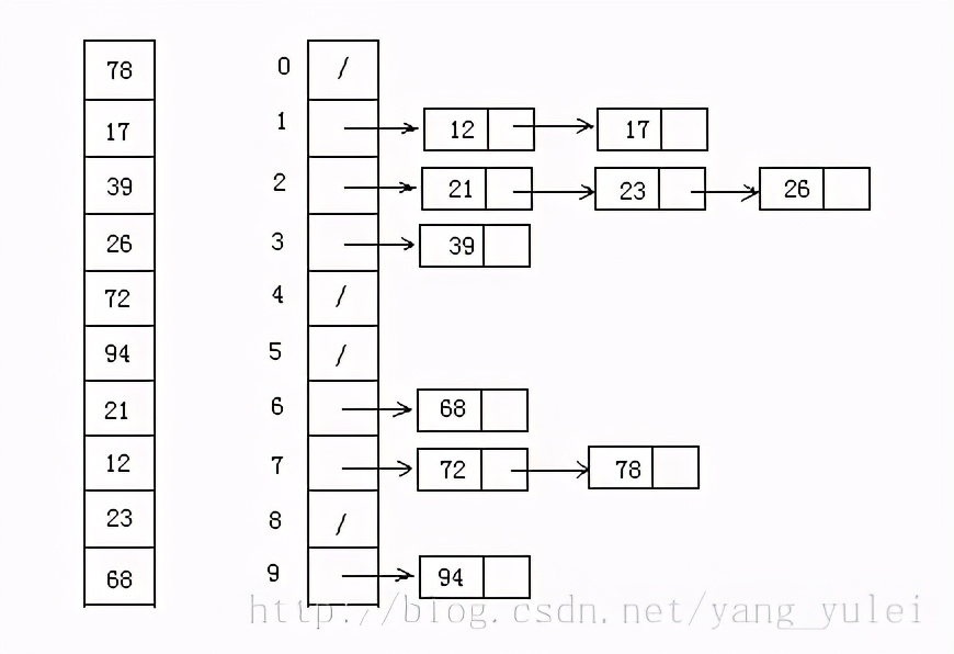
9. Bucket Sort

Bucket sorting is an upgraded version of counting sorting. It makes use of the mapping relationship of the function. The key to efficiency lies in the determination of the mapping function.

Working principle of bucket sort: assuming that the input data is uniformly distributed, divide the data into a limited number of buckets, and sort each bucket separately (it is possible to use another sorting algorithm or continue to use bucket sorting recursively)

9.1 algorithm description

• Manually set a bucket size as how many different values can be placed in each bucket (for example, when bucket size = = 5, the bucket can store {1,2,3,4,5} numbers, but the capacity is unlimited, that is, 100 3 can be stored);
• Traverse the input data and put the data into the corresponding bucket one by one;
• To sort each bucket that is not empty, you can use other sorting methods or recursive bucket sorting;
• Splice the ordered data from a bucket that is not empty.

Note that if bucket sorting is used recursively to sort each bucket, when the bucket number is 1, manually reduce the bucket size and increase the number of buckets in the next cycle, otherwise it will fall into an endless loop, resulting in memory overflow.

9.2 picture presentation

9.3 code implementation

    /**
     * Bucket sorting
     * 
     * @param array
     * @param bucketSize
     * @return
     */
    public static ArrayList<Integer> BucketSort(ArrayList<Integer> array, int bucketSize) {
        if (array == null || array.size() < 2)
            return array;
        int max = array.get(0), min = array.get(0);
        // Max min found
        for (int i = 0; i < array.size(); i++) {
            if (array.get(i) > max)
                max = array.get(i);
            if (array.get(i) < min)
                min = array.get(i);
        }
        int bucketCount = (max - min) / bucketSize + 1;
        ArrayList<ArrayList<Integer>> bucketArr = new ArrayList<>(bucketCount);
        ArrayList<Integer> resultArr = new ArrayList<>();
        for (int i = 0; i < bucketCount; i++) {
            bucketArr.add(new ArrayList<Integer>());
        }
        for (int i = 0; i < array.size(); i++) {
            bucketArr.get((array.get(i) - min) / bucketSize).add(array.get(i));
        }
        for (int i = 0; i < bucketCount; i++) {
            if (bucketSize == 1) { // If there are duplicate numbers in the sorted array, thank @ see the wind, but the wind friend points out the error
                for (int j = 0; j < bucketArr.get(i).size(); j++)
                    resultArr.add(bucketArr.get(i).get(j));
            } else {
                if (bucketCount == 1)
                    bucketSize--;
                ArrayList<Integer> temp = BucketSort(bucketArr.get(i), bucketSize);
                for (int j = 0; j < temp.size(); j++)
                    resultArr.add(temp.get(j));
            }
        }
        return resultArr;
    }

9.4 algorithm analysis

In the best case of bucket sorting, linear time O(n) is used. The time complexity of bucket sorting depends on the time complexity of sorting the data between buckets, because the time complexity of other parts is O(n). Obviously, the smaller the bucket is divided, the less the data between buckets, and the less the sorting time will be. But the corresponding space consumption will increase.

Best case: T(n) = O(n+k) worst case: T(n) = O(n+k) average case: T(n) = O(n2)

10. Radix Sort

Cardinality sorting is also a non comparison sorting algorithm. Each bit is sorted from the lowest bit. The complexity is O(kn), which is the length of the array, and k is the maximum number of digits in the array;

Cardinality sorting is to sort first according to the low order and then collect; then sort according to the high order and then collect; and so on until the highest order. Sometimes some attributes have priority order, sort according to the low priority first, and then sort according to the high priority. The last order is the high priority first, and the low priority with the same high priority first. Cardinality sorting is based on score Do not sort, collect separately, so it is stable.

10.1 algorithm description

• Get the maximum number in the array and get the number of bits;
• arr is the original array, and each bit is taken from the lowest bit to form a radius array;
• Count and sort the radix (using the characteristics that count sorting is suitable for a small range of numbers);

10.2 dynamic diagram demonstration

10.3 code implementation

　　/**
     * Cardinality sort
     * @param array
     * @return
     */
    public static int[] RadixSort(int[] array) {
        if (array == null || array.length < 2)
            return array;
        // 1. First calculate the number of digits of the maximum number;
        int max = array[0];
        for (int i = 1; i < array.length; i++) {
            max = Math.max(max, array[i]);
        }
        int maxDigit = 0;
        while (max != 0) {
            max /= 10;
            maxDigit++;
        }
        int mod = 10, div = 1;
        ArrayList<ArrayList<Integer>> bucketList = new ArrayList<ArrayList<Integer>>();
        for (int i = 0; i < 10; i++)
            bucketList.add(new ArrayList<Integer>());
        for (int i = 0; i < maxDigit; i++, mod *= 10, div *= 10) {
            for (int j = 0; j < array.length; j++) {
                int num = (array[j] % mod) / div;
                bucketList.get(num).add(array[j]);
            }
            int index = 0;
            for (int j = 0; j < bucketList.size(); j++) {
                for (int k = 0; k < bucketList.get(j).size(); k++)
                    array[index++] = bucketList.get(j).get(k);
                bucketList.get(j).clear();
            }
        }
        return array;
    }

10.4 algorithm analysis

Best case: T(n) = O(n * k) worst case: T(n) = O(n * k) average case: T(n) = O(n * k)

There are two methods of cardinality sorting:

MSD starts sorting from high order and LSD starts sorting from low order

Cardinality sort vs count sort vs bucket sort

These three sorting algorithms all use the concept of bucket, but there are obvious differences in the use of bucket:

• Cardinality sorting: allocate buckets according to each number of key value
• Count sorting: each bucket stores only one key value
• Bucket sorting: each bucket stores a certain range of values

Source:
https://www.cnblogs.com/guoyaohua/p/8600214.html

Reply to cxuan under my official account cxuan, and receive the following PDF, write it yourself.