Starting from this article, the author officially began to explain the knowledge related to Python in-depth learning, neural network and artificial intelligence. I hope you like it.
The previous article explained the installation process of TensorFlow and the basic concepts of neural network. This article will share the basis of TensorFlow and introduce the case of univariate linear prediction, mainly combined with the author's previous blog and the video introduction of "don't bother God". Later, we will explain the specific projects and applications in depth.
Basic articles, I hope to help you. If there are errors or deficiencies in the articles, please Haihan ~ at the same time, I am also a rookie of artificial intelligence. I hope you can grow up with me in this stroke by stroke blog.
Article directory:
- 1, Neural network Preface
- 2, TensorFlow structure and working principle
- 3, TensorFlow to realize univariate linear prediction
- 4, Summary
Code download address (welcome to pay attention and praise):
- https://github.com/eastmountyxz/ AI-for-TensorFlow
- https://github.com/eastmountyxz/ AI-for-Keras
1, Neural network Preface
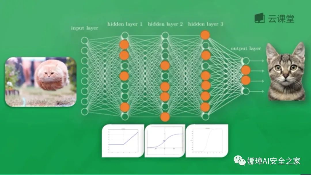
As shown in the figure below, animals, cats or dogs are identified through the neural network, including Input Layer, Hidden Layer and Output Layer. Each neuron has an excitation function. The information transmitted by the excited neuron is the most valuable. It also determines the final output result. After massive data training, the neural network can be used to identify cats or dogs.
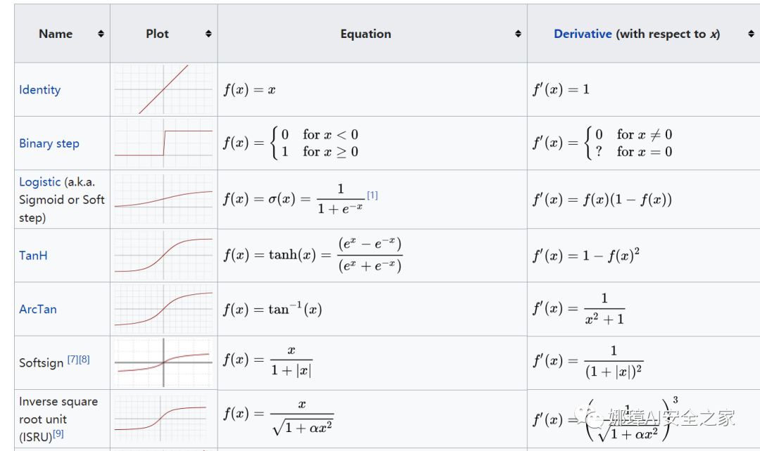
The excitation function is equivalent to a filter or exciter, which activates unique information or features. Common activation functions include softplus, sigmoid, relu, softmax, elu, tanh, etc. For hidden layers, we can use nonlinear relations such as relu, tanh and softplus; For the classification problem, we can use sigmoid (the smaller the value is, the closer it is to 0, and the larger the value is, the closer it is to 1) and softmax function to calculate the probability for each class, and finally take the maximum probability as the result; For regression problems, linear function can be used to experiment.
All neurons in the neural network have activation function s. For common excitation functions, please refer to Wikipedia:
- https://en.wikipedia.org/wiki/ Activation_function
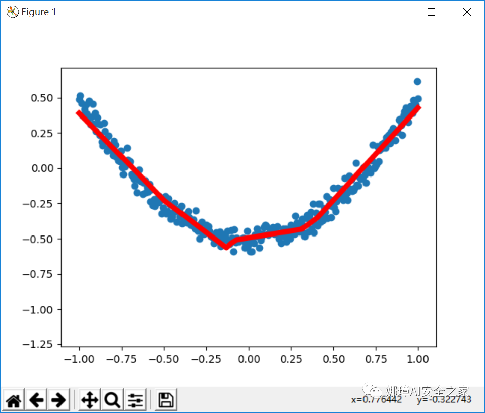
Now suppose that the input x represents a string of numbers, the output y represents a quadratic function, the blue point represents the data set, and the red line represents a curve learned by the neural network and represents our data. At first, this curve may be tortuous. With continuous training and learning, this curve will gradually fit to my data. The more the red line conforms to the trend of data, the more things the neural network learns and the more it can predict its trend.
2, TensorFlow structure and principle
What is Tensorflow?
Tensorflow is an open source software library that uses data flow graphs technology for numerical calculation. Data flow graph is a directed graph, which uses nodes (generally described by circles or squares, representing the starting point of a mathematical operation or data input and the end point of data output) and lines (representing numbers, matrices or Tensor tensors) to describe mathematical calculations.
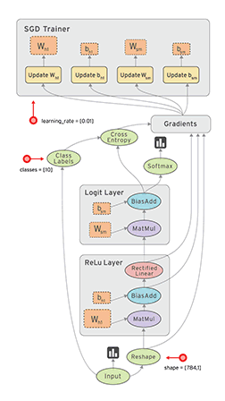
Data flow graph can easily allocate each node to different computing devices to complete asynchronous parallel computing, which is very suitable for large-scale machine learning applications [7]. As shown in the figure below, we continuously learn and improve our weight W and offset b through Gradients, so as to improve the accuracy.
TensorFlow supports various heterogeneous platforms, supports multiple CPUs / GPUs, servers and mobile devices, and has good cross platform characteristics; TensorFlow has flexible architecture, can support various network models, and has good universality.
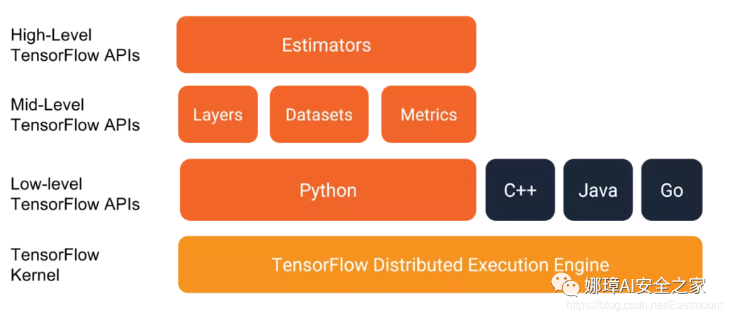
In addition, TensorFlow kernel is developed in C/C + +, and provides client APIs in C + +, Python, Java and Go languages. Its architecture is flexible, can support various network models, and has good universality and scalability. tensorflow.js supports running GPU training depth learning model on the web using webGL, and supports loading and running machine learning model in IOS and Android systems. Its basic structure is shown in the figure below:
How does TensorFlow process data?
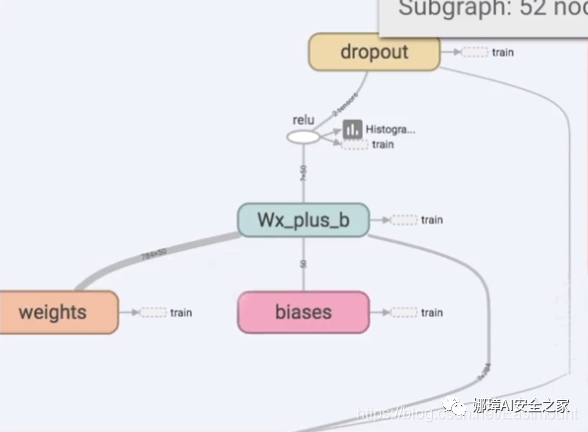
Next, let's share Mr. Mofan's analysis of TensorFlow's working principle. The following figure is a typical neural network structure including input layer, hidden layer and output layer.
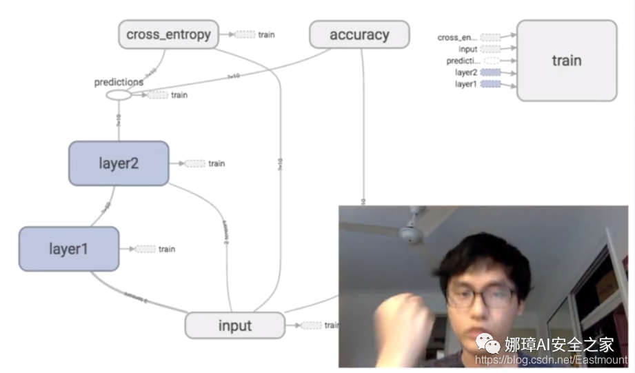
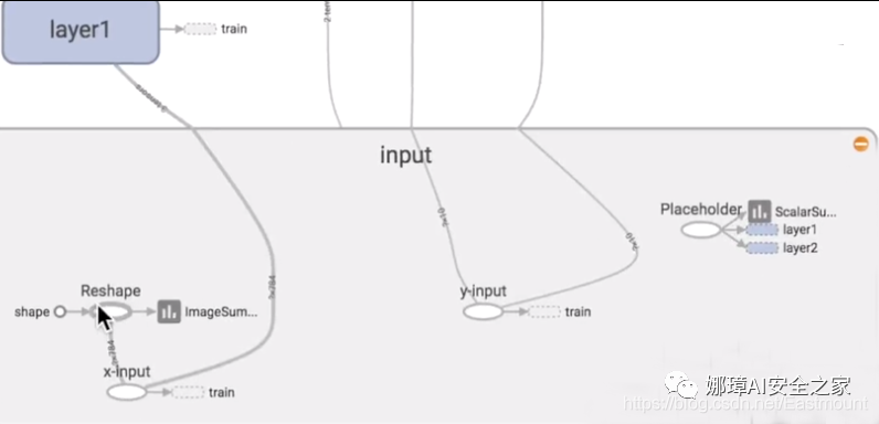
Click the input layer and find that it contains x-input and y-input; Then, the hidden layer contains weights and biases, as well as an excitation function relu, which will be shared later.
What is the first step in TensorFlow?
It needs to establish such a structure, then put the data into this structure, let TensorFlow run by itself, and output accurate prediction results through continuous training, learning and modifying parameters. TensorFlow Chinese translation is "vector flies in this structure", which is also the basic meaning of TensorFlow.
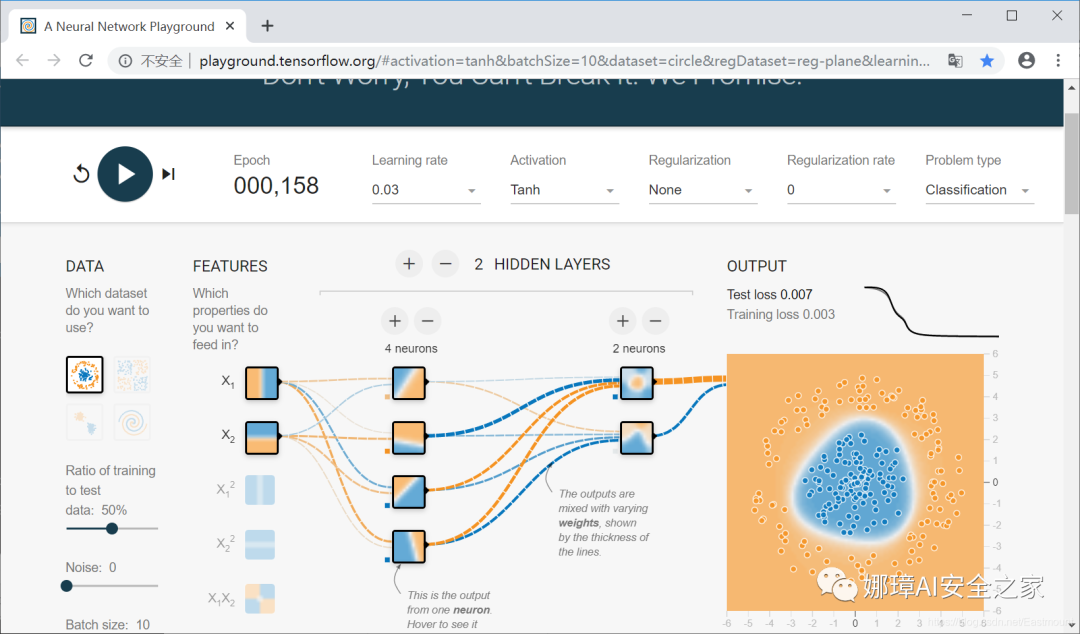
Finally, an online neural network simulator is added. You can try to run it to see the working principle and parameter adjustment of neural network. The address is:
- http://playground.tensorflow.org/
3, TensorFlow univariate linear prediction
Then, a case of TensorFlow predicting linear line (y = 0.1 * x + 0.3) is added.
1. First, define 100 randomly generated numbers and linear lines The more common format in TensorFlow is float32, which is also set here. At the same time, the predicted weight is 0.1 and the bias is 0.3
x_data = np.random.rand(100).astype(np.float32) print(x_data) y_data = x_data * 0.1 + 0.3 print(y_data)
The output result is:
[0.42128456 0.3590797  0.31952253 0.54071575 0.4098252  0.87536865
 0.58871204 0.37161928 0.30826327 0.94290715 0.40412208 0.47935355
 ...
 0.00465394 0.0929272  0.18561055 0.8577836  0.6737635  0.04606532
 0.8738483  0.9900948  0.13116711 0.299359  ]
[0.34212846 0.335908   0.33195227 0.3540716  0.34098253 0.38753688
 0.35887122 0.33716193 0.33082634 0.39429075 0.34041223 0.34793538
...
 0.3004654  0.30929273 0.31856108 0.38577837 0.36737636 0.30460656
 0.38738483 0.3990095  0.31311673 0.3299359 ]
2. Create TensorFlow structure and define Weights and bias The weight is tf.Variable parameter variable, and the one-dimensional structure sequence is randomly generated, with the range of - 1.0 to 1.0; The initial value of offset bias is 0. The purpose of TensorFlow learning is to continuously improve from the initial value to goals 0.1 (Weights) 0 and 0.3 (bias).
Weights = tf.Variable(tf.random_uniform([1], -1.0, 1.0)) print(Weights) biases = tf.Variable(tf.zeros([1])) print(biases)
The output result is:
<tf.Variable 'Variable_28:0' shape=(1,) dtype=float32_ref>
<tf.Variable 'Variable_29:0' shape=(1,) dtype=float32_ref>
3. Define the predicted value y and loss function The loss function is the predicted y and the actual y_ Minimum variance of data.
y = Weights * x_data + biases loss = tf.reduce_mean(tf.square(y-y_data))
4. Construct neural network optimizer (gradient descent optimization function) The optimizer here is GradientDescentOptimizer, which reduces the error through the optimizer, reduces the error in each step of training and improves the parameter accuracy. The learning efficiency is set to 0.5, which is generally a number less than 1.
optimizer = tf.train.GradientDescentOptimizer(learning_rate=0.5) train = optimizer.minimize(loss)
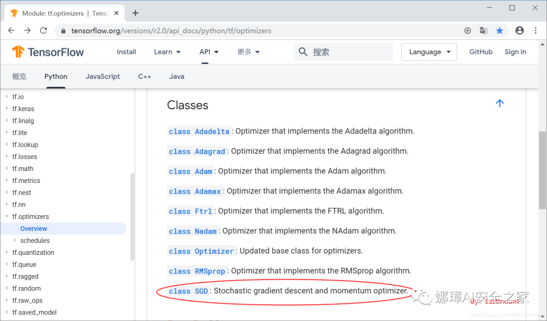
Note that some methods of tensorflow 2.0 and tensorflow 1.0 have been changed. For example, in the case of predicting house prices in California, the tf.train.Gradient Descent Optimizer class is no longer available. The train module is removed by 2.0 as a whole. The comparison is as follows.
- TensorFlow1.0: optimizer = tf.train.GradientDescentOptimizer(0.5)
- TensorFlow2.0: optimizer = tf.optimizers.SGD(learning_rate=0.5)
Please check the official documents for more methods. The author wanted to explain with tensorflow 2.0, but found that there were too many changes. I'm going to start with tensorflow 1.0. Later, with my in-depth study and understanding, I'll share the code of tensorflow 2.0. Please forgive me.
TF2.0 official:
- https://www.tensorflow.org/versions/ r2.0/api_docs/python/tf/optimizers
In TensorFlow 2.0, Keras became the default high-level API, and optimizer functions migrated from tf.keras.optimizers into separate API called tf.optimizers. They inherit from Keras class Optimizer. Relevant functions from tf.train aren't included into TF 2.0. So to access GradientDescentOptimizer, call tf.optimizers.SGD
5. Initialize variables
init = tf.global_variables_initializer()
6. Define Session and train, and output results every 20 times
# Define Session
sess = tf.Session()
# The runtime Session is like a pointer to the location to be processed and activated
sess.run(init)t
# Training 201 times
for n in range(201):
    # Train and output the results every 20 times
    sess.run(train)
    if n % 20 == 0:
        # Best fitting result W: [0.100], b: [0.300]
        print(n, sess.run(Weights), sess.run(biases))
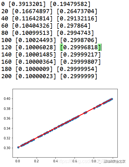
The output results are shown in the figure below. Its parameters weight and bias are output every 20 training sessions. What we want to do is to predict the linear line. At first, the calculated value and the test value will be very different. What the neural network needs to do is to continuously reduce the predicted value y and the actual value y_data differences. Finally, after 200 training, we are very close to these scattered points.
0 [-0.17100081] [0.60644317]
20 [0.00904198] [0.34798568]
40 [0.07555631] [0.31289548]
60 [0.09343112] [0.3034655]
80 [0.09823472] [0.3009313]
100 [0.09952562] [0.3002503]
120 [0.09987252] [0.30006728]
140 [0.09996576] [0.30001807]
160 [0.09999081] [0.30000487]
180 [0.09999753] [0.30000132]
200 [0.09999932] [0.30000037]
7. Visual display
pre = x_data * sess.run(Weights) + sess.run(biases) plt.scatter(x_data, y_data) plt.plot(x_data, pre, 'r-') plt.show()
The complete code is as follows (simplified version):
# -*- coding: utf-8 -*-
"""
Created on 2019-11-30 Written at Wuhan University at 6 p.m
@author: Eastmount CSDN YXZ
"""
import tensorflow as tf
import numpy as np
import matplotlib.pyplot as plt
import time

x_data = np.random.rand(100).astype(np.float32)
y_data = x_data * 0.1 + 0.3 #Weight 0.1 offset 0.3

#------------------Start creating tensorflow structure------------------
# Weights and offsets
Weights = tf.Variable(tf.random_uniform([1], -1.0, 1.0))
biases = tf.Variable(tf.zeros([1]))

# Predicted value y
y = Weights * x_data + biases

# loss function
loss = tf.reduce_mean(tf.square(y-y_data))

# Establish neural network optimizer
optimizer = tf.train.GradientDescentOptimizer(learning_rate=0.5) #learning efficiency
train = optimizer.minimize(loss)

# initialize variable
init = tf.global_variables_initializer()
#------------------End creating tensorflow structure------------------

# Define Session
sess = tf.Session()

# The runtime Session is like a pointer to the location to be processed and activated
sess.run(init)

# Train and output the results every 20 times
for n in range(201):
    sess.run(train)
    if n % 20 == 0:
        print(n, sess.run(Weights), sess.run(biases))
        pre = x_data * sess.run(Weights) + sess.run(biases)

# Visual analysis
plt.scatter(x_data, y_data)
plt.plot(x_data, pre, 'r-')
plt.show()
The output results are shown in the figure below. The weight is gradually optimized from the initial random number of 0.3913201 to the target of 0.1; The bias is gradually optimized from the initial random number of 0.19479582 to 0.3 through continuous learning and training.
8. Complete code for visual comparison of multiple renderings
# -*- coding: utf-8 -*-
"""
Created on Sun Dec 1 20:00:14 2019
@author: xiuzhang Eastmount
"""
import tensorflow as tf
import numpy as np
import matplotlib.pyplot as plt
x_data = np.random.rand(100).astype(np.float32)
y_data = x_data * 0.1 + 0.3 #Weight 0.1 offset 0.3
#------------------Start creating tensorflow structure------------------
# Weights and offsets
Weights = tf.Variable(tf.random_uniform([1], -1.0, 1.0))
biases = tf.Variable(tf.zeros([1]))
# Predicted value y
y = Weights * x_data + biases
# loss function
loss = tf.reduce_mean(tf.square(y-y_data))
# Establish neural network optimizer
optimizer = tf.train.GradientDescentOptimizer(learning_rate=0.5) #learning efficiency
train = optimizer.minimize(loss)
# initialize variable
init = tf.global_variables_initializer()
#------------------End creating tensorflow structure------------------
# visualization
plt.plot(x_data, y_data,'ro', marker='^', c='blue',label='original_data')
plt.legend()
plt.show()
# Define Session
sess = tf.Session()
# The runtime Session is like a pointer to the location to be processed and activated
sess.run(init)
# Train and output the results every 20 times
k = 0
for n in range(200):
sess.run(train)
if n % 20 == 0:
print(n, sess.run(Weights), sess.run(biases))
pre = x_data * sess.run(Weights) + sess.run(biases)
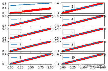
# Visual analysis
k = k + 1
plt.subplot(5, 2, k)
plt.plot(x_data, y_data, 'ro')
plt.plot(x_data, pre, label=k)
plt.legend()
plt.show()
The output results are shown in the figure below:
4, Summary
This is the end of this basic TensorFlow article. Through continuous training and learning, it matches the predicted results with the actual curve y=0.1*x+0.3. This is a very basic in-depth learning article. At the same time, if there are errors or deficiencies in the article, please forgive me
References, thank you for your articles and videos. I recommend you to follow Mr. Mo fan. He is my introductory teacher of artificial intelligence.
- [1] Introduction to neural networks and machine learning - author's article
- [2] Stanford machine learning video Professor NG: https://class.coursera.org/ml/class/index
- [3] Book "artificial intelligence in game development"
- [4] Netease cloud don't bother teacher video (strong push): https://study.163.com/course/courseLearn.htm?courseId=1003209007
- [5] Neural network excitation function - deep learning
- [6] tensorflow Architecture - NoMorningstar
- [7] Tensorflow 2.0 introduction to low level api - GumKey
- [8] https://tensorflow.google.cn/overview/
- [9] http://playground.tensorflow.org/
- [10] https://www.tensorflow.org/versions/ r2.0/api_docs/python/tf/optimizers