Project description

The data is tiktok's interaction record from 9-21 to 10-30 days. The year has been processed for special treatment (2067 shows).
·The first column is not marked (such as sequence ID, but it is discontinuous. It is estimated that the data set has been filtered)
·uid: user id
·user_city: user's City
·item_id: work id
·Author id: author id
·item_city: City
·channel: the source of the work
·Finish: finish browsing the work
·Like: do you like your work
·music id: music id
·Device: device id
·Time: release time of the work
·duration time: duration s

Analysis purpose: to put forward suggestions on the operation of network red and platform

data processing

import pandas as pd
import numpy as np
import time
from pyecharts.charts import Line,Pie,Grid,Bar,Page
import pyecharts.options as opts
from bs4 import BeautifulSoup

data=pd.read_table('douyin.txt',header=None)
#Supplementary value field name
data.columns = ['uid','user_city','item_id','author_id','item_city','channel','finish','like','music_id','device','time','duration_time']
data.head()

data.info()

Missing value processing

There are no missing values

data.isnull().sum()

Duplicate value processing

#Delete duplicate values
print('Number of duplicate values:',data.duplicated().sum())
data.drop_duplicates(inplace=True)

Number of duplicate values: 4924

#The data is desensitized data, and the original situation cannot be observed. However, it can be inferred that - 1 is the missing value, which can be deleted directly after conversion.
data[data==-1] = np.nan
data.dropna(inplace=True)

#The device column and the extra Unnamed: 0 column will not be used in this analysis. Delete them
del data['device']

data conversion

#The time column is the timestamp, which is modified to the normal time
data.time=data.time.astype('str')\
                    .apply(lambda x:x[1:])\
                    .astype('int64')

#Convert timestamp to normal date format
real_time = []
for i in data['time']:
    stamp = time.localtime(i)
    strft = time.strftime("%Y-%m-%d %H:%M:%S", stamp)
    real_time.append(strft)
    
data['real_time'] = pd.to_datetime(real_time)

#The time column is useless. Delete it
del data['time']

#Add H: hour, and date: Date columns to the data
data['H'] = data.real_time.dt.hour
data['date']=data.real_time.dt.date
data=data[data.real_time>pd.to_datetime('2067-09-20')]

data.head()

Data analysis

Daily broadcast volume, user volume, author volume and contribution volume

#Daily playback volume
ids=data.groupby('date')['date'].count()
#Daily user volume
uids=data.groupby('date')['uid'].nunique()
#Daily author volume
author=data.groupby('date')['author_id'].nunique()
#Daily production
items=data.groupby('date')['item_id'].nunique()

#Daily playback volume
line1 = (
    Line()
    .add_xaxis(ids.index.tolist())
    .add_yaxis('Daily playback volume', ids.values.tolist())
    .set_global_opts(
        title_opts=opts.TitleOpts(title='Change trend of daily playback volume',pos_left="20%"),
        legend_opts=opts.LegendOpts(is_show=False),
        yaxis_opts=opts.AxisOpts(name='Daily playback volume'),
    )
    .set_series_opts (label_opts=opts.LabelOpts(is_show=False))
)


#Daily user volume
line2 = (
    Line()
    .add_xaxis(uids.index.tolist())
    .add_yaxis('Daily user volume', uids.values.tolist())
    .set_global_opts(
        title_opts=opts.TitleOpts(title='Change trend of daily user volume',pos_right="20%"),
        legend_opts=opts.LegendOpts(is_show=False),
         yaxis_opts=opts.AxisOpts(name='Daily user volume'),
    )
    .set_series_opts (label_opts=opts.LabelOpts(is_show=False))
)


#Daily author volume
line3 = (
    Line()
    .add_xaxis(author.index.tolist())
    .add_yaxis('Daily author volume', author.values.tolist())
    .set_global_opts(
        title_opts=opts.TitleOpts(title='Change trend of daily author volume',pos_top="50%",pos_left="20%"),
        legend_opts=opts.LegendOpts(is_show=False),
        yaxis_opts=opts.AxisOpts(name='Daily author volume'),
    )
    .set_series_opts (label_opts=opts.LabelOpts(is_show=False))
)


#Daily production
line4 = (
    Line()
    .add_xaxis(items.index.tolist())
    .add_yaxis('Daily contributions', items.values.tolist())
    .set_global_opts(
        title_opts=opts.TitleOpts(title='Change trend of daily contribution',pos_top="50%", pos_right="20%"),
        legend_opts=opts.LegendOpts(is_show=False),
        yaxis_opts=opts.AxisOpts(name='Daily contributions'),
    )
    .set_series_opts (label_opts=opts.LabelOpts(is_show=False))
)

grid1 = (
    Grid()
    .add(line1, grid_opts=opts.GridOpts(pos_bottom="60%",pos_right="55%"))
    .add(line2, grid_opts=opts.GridOpts(pos_bottom="60%",pos_left="55%"))
    .add(line3, grid_opts=opts.GridOpts(pos_top="60%",pos_right="55%"))
    .add(line4, grid_opts=opts.GridOpts(pos_top="60%",pos_left="55%"))
)

grid1.render_notebook()

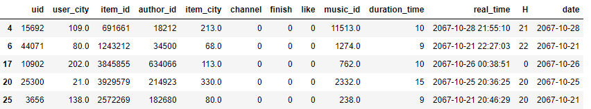
Before October 21, the change trend of daily broadcast volume, daily user volume, daily author volume and daily contribution volume with time is basically the same: steady growth;
During the period from 10-21 to 10-30, all indicators first show a huge growth, then tend to be stable, and then fall back to the normal level. It is guessed that the platform has carried out promotion activities at this time point.

However, it can be clearly seen that the increase in the number of users is not exaggerated. And the number of authors and contributions has also increased rapidly compared with the number of users. The preliminary guess is that someone took advantage of the loopholes in the platform rules to create a large number of new numbers and use robots to brush bills for profit.
Unfortunately, it is difficult to evaluate the effect of this activity because there is no data for a longer period. However, you can try to check out the robot account.

exception=data.groupby(['uid','date'])['uid'].count()[data.groupby(['uid','date'])['uid'].count()>1].unstack().T
exception.index=exception.index.astype('datetime64[ns]')
exception.head()

#(forecast) change times of average viewing per person before and after the activity starts
times = exception.query('date>datetime(2067,10,21) and date<datetime(2067,10,29)').mean() / exception.query('date<datetime(2067,10,21)').mean()

times.describe([0.25,0.5,0.75,0.8,0.85,0.9,0.95,0.99])

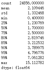
#Robot (the change multiple of most people is between 0-3 times, so 3 times is selected)
robot = times[times>3].index.tolist()
len(robot)

4267

new=data.query('real_time>datetime(2067,10,21) & real_time<datetime(2067,10,29)')['uid']
old=data.query('real_time<datetime(2067,10,21)')['uid']
print('10-21 To 10-29 The number of new users in daily activities is:',new.nunique()-new[new.isin(old)].nunique())

The number of new users from October 21 to October 29 is 5739
Conclusion: 4267 of the robots are suspected, and the new users are 5739. This further confirms that the current network is mainly based on the stock market. If we want to attract new creators and users, we may need to go to new markets, such as overseas or in the market outside the tiktok market.

Playback source distribution

channel = data.groupby('channel')['uid'].count()

pie1=(
      Pie()
     .add('Playback volume', [list(z) for z in zip(channel.index.tolist(), channel.values.tolist())])
     .set_global_opts(title_opts=opts.TitleOpts(title='Playback source distribution',pos_left='20%'),legend_opts=opts.LegendOpts(is_show=False))
     .set_series_opts(label_opts=opts.LabelOpts(formatter="{b}:{d}%"))
      )
pie1.render_notebook()

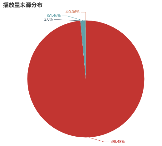
Although there is no clear explanation, as an algorithm driven short video platform, it is obvious that "0" is the video recommended by the algorithm. The key to get the volume of the play is to get the algorithm tiktok into the larger flow pool.

Work duration

#Duration and playback volume of works
duration_uid = data.groupby('duration_time')['uid'].count()

#View the relationship between the duration and the completion rate and the like rate
time_finish = data[['duration_time','finish','like']].groupby('duration_time').mean()

#Only works with more than 100 plays in each duration are counted
num_100=time_finish[data[['duration_time','finish','like']].groupby('duration_time').count()>100]
num_100.dropna(inplace=True)

#Duration and number of works
duration_nums = data.groupby('duration_time')['item_id'].nunique()

line5=(
    Line()
    .add_xaxis(duration_uid.index.tolist())
    .add_yaxis('Playback volume', duration_uid.values.tolist())
    .set_global_opts(
        title_opts=opts.TitleOpts(title='Relationship between work duration and playback volume',pos_left="15%"),
        legend_opts=opts.LegendOpts(is_show=False),
        yaxis_opts=opts.AxisOpts(name='Playback volume'),
                      )
    .set_series_opts (label_opts=opts.LabelOpts(is_show=False))
    )

line6=(
    Line()
    .add_xaxis(duration_nums.index.tolist())
    .add_yaxis('Number of submissions', duration_nums.values.tolist())
    .set_global_opts(
        title_opts=opts.TitleOpts(title='The relationship between the length of work and the number of contributions',pos_right="15%"),
        legend_opts=opts.LegendOpts(is_show=False),
        yaxis_opts=opts.AxisOpts(name='Number of submissions'),
                      )
    .set_series_opts (label_opts=opts.LabelOpts(is_show=False))
    )

line7=(
    Line()
    .add_xaxis(num_100.index.tolist())
    .add_yaxis('Completion rate', num_100.finish.tolist())
    .set_global_opts(
        title_opts=opts.TitleOpts(title='Relationship between work duration and completion rate',pos_top="50%",pos_left="15%"),
        legend_opts=opts.LegendOpts(is_show=False),
        yaxis_opts=opts.AxisOpts(name='Completion rate',min_=0.35,max_=0.55),
                      )
    .set_series_opts (label_opts=opts.LabelOpts(is_show=False))
    )

line8=(
    Line()
    .add_xaxis(num_100.index.tolist())
    .add_yaxis('Praise rate', num_100.like.tolist())
    .set_global_opts(
        title_opts=opts.TitleOpts(title='Relationship between work duration and praise rate',pos_top="50%", pos_right="15%"),
        legend_opts=opts.LegendOpts(is_show=False),
        yaxis_opts=opts.AxisOpts(name='Praise rate',min_=0.004,grid_index=4),
                      )
    .set_series_opts (label_opts=opts.LabelOpts(is_show=False))
    )

grid2 = (
    Grid()
    .add(line5, grid_opts=opts.GridOpts(pos_bottom="60%",pos_right="55%"))
    .add(line6, grid_opts=opts.GridOpts(pos_bottom="60%",pos_left="55%"))
    .add(line7, grid_opts=opts.GridOpts(pos_top="60%",pos_right="55%"))
    .add(line8, grid_opts=opts.GridOpts(pos_top="60%",pos_left="55%"))
)

grid2.render_notebook()

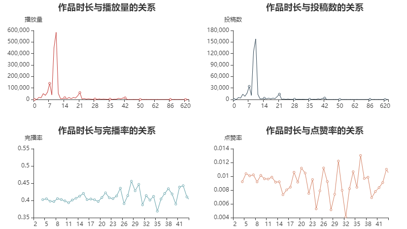
Observations:
The duration of most works is between 7-10s. Generally speaking, there are a certain number of submissions between 0s-22s, and few more than 22s.
The duration distribution of playback volume is basically the same as that of the number of works.
The completion rate is generally more than 40% within 2s-27s, and fluctuates violently between 37% - 45% after 27s,
The praise rate is basically maintained within 1% in 2s-14s, and fluctuates between 0.7% - 1.1% in 14s-20s. After 20s, the fluctuation of data changes is completely irregular.

Conclusion: the best video duration is 7-10s, followed by 0-6s and 23s, and the longest is not recommended to exceed 40s (none of the records exceeds 50s, and the video playback volume exceeds 100)

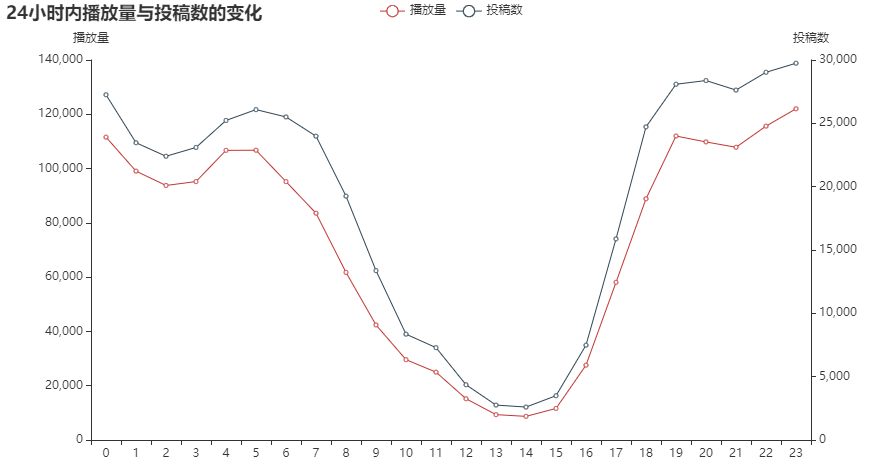
Each hour

#Playback volume per hour
H_num = data.groupby('H')['uid'].count()
#Number of submissions per hour
H_item = data.groupby('H')['item_id'].nunique()
#Relationship between the release time of works and the completion rate of likes
H_f_l = data.groupby('H')[['finish','like']].mean()

line9=(
    Line()
    .add_xaxis(H_num.index.tolist())
    .add_yaxis('Playback volume', H_num.values.tolist())
    .extend_axis(yaxis=opts.AxisOpts(name="Number of submissions",position="right")) #min_=0,max_=25,
    .set_global_opts(
        title_opts=opts.TitleOpts(title='24 Changes in playback volume and submission number within hours'),
        yaxis_opts=opts.AxisOpts(name="Playback volume"), #,min_=0.35
                      )
    .set_series_opts (label_opts=opts.LabelOpts(is_show=False))
    )


line10=(
    Line()
    .add_xaxis(H_item.index.tolist())
    .add_yaxis('Number of submissions', H_item.values.tolist(),yaxis_index=1)
    .set_series_opts (label_opts=opts.LabelOpts(is_show=False))
    )

overlap1=line9.overlap(line10)
overlap1.render_notebook()

line11=(
    Line()
    .add_xaxis(H_f_l.index.tolist())
    .add_yaxis('finish', H_f_l.finish.tolist())
    .extend_axis(yaxis=opts.AxisOpts(name="Praise rate",position="right",min_=0.008)) 
    .set_global_opts(
        title_opts=opts.TitleOpts(title='Relationship between the release time of works and the completion rate of likes'),
        yaxis_opts=opts.AxisOpts(name="Completion rate",min_=0.35),
                      )
    .set_series_opts (label_opts=opts.LabelOpts(is_show=False))
    )


line12=(
    Line()
    .add_xaxis(H_f_l.index.tolist())
    .add_yaxis('like', H_f_l.like.tolist(),yaxis_index=1)
    .set_series_opts (label_opts=opts.LabelOpts(is_show=False))
    )

overlap2=line11.overlap(line12)
overlap2.render_notebook()

Conclusion: the overall playback volume and the number of submissions are basically the same, and the playback volume will be slightly higher from 19 p.m. to 5 p.m. the next day. There will not be much change in the praise rate and completion rate of works released in different time periods.
If the best time for submission is from 19:00 p.m. to 5:00 the next day, there is no special advantage in the completion rate and praise rate.

background music

#Difference in playing volume of top 100 popular songs
music_100=data.groupby('music_id')['uid'].count().sort_values(ascending=False).iloc[:100,].sort_values(ascending=False)

#Cumulative percentage distribution of total background music playback
music_cum=data['music_id'].value_counts().sort_values(ascending=False).cumsum()/len(data['uid'])
x=range(len(music_cum)+1)
line13 = (
    Line()
    .add_xaxis(x)
    .add_yaxis('Proportion of cumulative playback', music_cum.values.tolist())
    .set_global_opts(
        title_opts=opts.TitleOpts(title='Change trend of proportion of cumulative music playback',pos_left="40%"),
        legend_opts=opts.LegendOpts(is_show=False),
        yaxis_opts=opts.AxisOpts(name='Proportion of cumulative playback'),
        xaxis_opts=opts.AxisOpts(name='Number of music'),
    )
    .set_series_opts (label_opts=opts.LabelOpts(is_show=False))
)
line13.render_notebook()

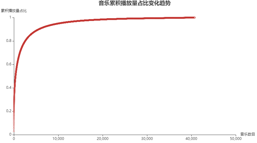
Conclusion: for video soundtrack, it is easier to recommend the hottest song at that time and get high playback volume than other songs.

#Like rate and completion rate of top ten songs
top_10=data.groupby('music_id')[['finish','like']].mean()\
     .loc[data.groupby('music_id')['uid'].count().sort_values(ascending=False).iloc[:10,].index.tolist()]\
     .sort_values('finish',ascending=False)
#Average completion rate and like rate of songs with playback volume greater than 10
avg_10=data.groupby('music_id')[['finish','like']].mean()[data.groupby('music_id')['uid'].count()>10].mean()

bar1=(
    Bar()
    .add_xaxis(top_10.index.tolist())
    .add_yaxis('finish', top_10.finish.tolist())
    .extend_axis(yaxis=opts.AxisOpts(name="Praise rate",position="right",min_=0.005))
    .add_yaxis('like', top_10.like.tolist(),yaxis_index=1)
    .set_global_opts(
        title_opts=opts.TitleOpts(title='Like rate and completion rate of top ten songs'),
        yaxis_opts=opts.AxisOpts(name="Completion rate",min_=0.38),
        )
    .set_series_opts (
        label_opts=opts.LabelOpts(is_show=False),
         markline_opts=opts.MarkLineOpts(
            data=[
                opts.MarkLineItem(name="Average completion rate",y = avg_10.finish),
                opts.MarkLineItem(name="Average praise rate",y = avg_10.like)
            ],
            label_opts=opts.LabelOpts(), #Do not display data labels          
        ),
                 )
    )


bar1.render_notebook()

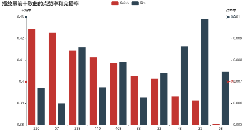
It can be seen that the like rate and completion rate of the most popular songs do not exceed the average. It can be seen that using popular songs can not improve their own like rate and completion rate.

#Change chart of daily playing volume of popular songs
top_date=data.groupby(['music_id','date'])['uid'].count()\
             .loc[data.groupby('music_id')['uid'].count().sort_values(ascending=False).iloc[:10,].index.tolist()]\
             .unstack().T

line14=(
    Line()
    .add_xaxis(top_date.index.tolist())
    .add_yaxis(str(top_date.columns[0]), top_date.iloc[:,:1].values.tolist())
    .add_yaxis(str(top_date.columns[1]), top_date.iloc[:,1:2].values.tolist())
    .add_yaxis(str(top_date.columns[2]), top_date.iloc[:,2:3].values.tolist())
    .add_yaxis(str(top_date.columns[3]), top_date.iloc[:,3:4].values.tolist())
    .add_yaxis(str(top_date.columns[4]), top_date.iloc[:,4:5].values.tolist())
    .add_yaxis(str(top_date.columns[5]), top_date.iloc[:,5:6].values.tolist())
    .add_yaxis(str(top_date.columns[6]),top_date.iloc[:,6:7].values.tolist())
    .add_yaxis(str(top_date.columns[7]), top_date.iloc[:,7:8].values.tolist())
    .add_yaxis(str(top_date.columns[8]), top_date.iloc[:,8:9].values.tolist())
    .add_yaxis(str(top_date.columns[9]), top_date.iloc[:,9:10].values.tolist())
    .set_global_opts(
        title_opts=opts.TitleOpts(title='Change trend of top ten songs',pos_left="38%"),
        legend_opts=opts.LegendOpts(pos_top='20%',pos_left='15%',orient='vertical'),
                      )
    .set_series_opts (label_opts=opts.LabelOpts(is_show=False))
    )
line14.render_notebook()

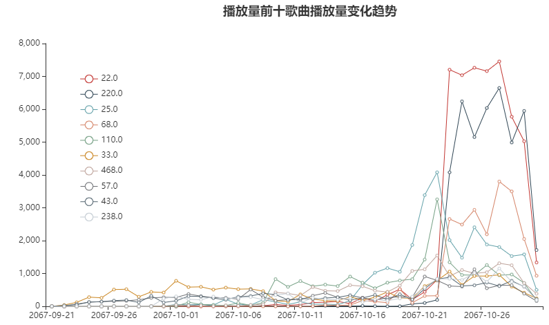
Within 10-21 to 10-29 days, the playback volume of each song has increased, among which the songs with ID 22220, 68 and 25 have a sharp upward trend.

Works and authors

#Cumulative distribution of total playback volume of each author id
item_cum=data['author_id'].value_counts().sort_values(ascending=False).cumsum()/len(data['uid'])
x=range(len(item_cum)+1)

line15 = (
    Line()
    .add_xaxis(x)
    .add_yaxis('Proportion of cumulative playback', item_cum.values.tolist())
    .set_global_opts(
        title_opts=opts.TitleOpts(title='Change trend of cumulative broadcast volume proportion of each author',pos_left="50%"),
        legend_opts=opts.LegendOpts(is_show=False),
        yaxis_opts=opts.AxisOpts(name='Proportion of cumulative playback'),
        xaxis_opts=opts.AxisOpts(name='Number of authors'),
    )
    .set_series_opts (label_opts=opts.LabelOpts(is_show=False))
)
line15.render_notebook()

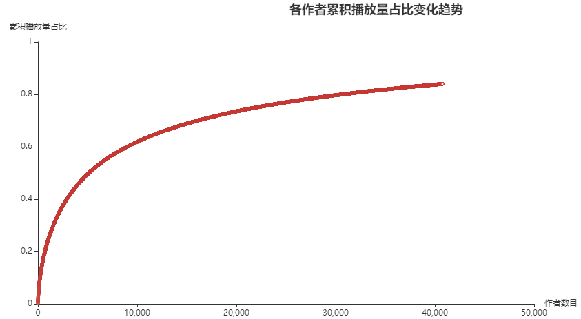
Conclusion: it can be seen that the current tiktok user play is very consistent with Pareto distribution, and a few producers have attracted most of the traffic of the platform. If you want to improve again on this basis, cultivating head producers or excavating head producers on other platforms is a more effective method than simply rewarding production. The specific effect needs more data support to draw a conclusion.

summary

Tiktok red recommendation

1. the flow of tiktok over 98% will flow to the algorithm recommended video, and the algorithm recommendation is the key to get more playback.
2. The video duration is preferably 7-10s, followed by 0-6s and 23s, and it is not recommended to exceed 40s.
3. The best submission time to get the playback volume is from 9 p.m. to 5 a.m. the next day, but there is no obvious time preference for the completion rate and praise rate.
4. It's best to choose the most popular songs to attract on-demand, but the most important thing is always the choice of theme.

Platform operation suggestions

1. there are many robots in the activity of shaking, and it needs to be determined whether to remove them (the [uid] of the tiktok is saved in the robot list).
2. The activities in the station are good at first, but there is no substantial growth after the removal of robots, and the income is very low. It needs to be careful to hold them again.
3. Platform users are always growing steadily, but if you want to grow a lot, it is better to consider other channels or open up new markets.
4. The top 20% of video producers account for more than 80% of the traffic of the whole platform. Cultivating or mining existing good video producers is the key to maintaining traffic in the future.

BI simple Kanban