The little teacher asked me to analyze the original data on the basis of the previously analyzed emotional data results. First, let me use PCA to reduce the dimension to see the data distribution, and then change TSNE to reduce the dimension.

It's really a small white wuwuwuwuwuwuwuwuwuwuwuwuwuwuwuwuwuwuwuwuwuwuwuwuwuwuwuwuwuwuwuwuwuwuwuwuwuwuwuwuwuwuwuwuwuwuwuwuwuwuwuwuwuwuwuwuwuwuwuwuwuwuwuwuwuwuwuwuwuwuwuwuwuwuwu

In this task, I learned to go to the official website for instructions if there are problems. For example, I use PCA sklearn.decomposition.PCA¶ Then go to the sklearn official website to find the function, and there are application examples of this function!

Then I chose PCA example with iris data set ¶   To learn from this example, refer to the link: PCA example with Iris Data-set — scikit-learn 1.0.1 documentation

Although the code is not much and you can understand it, Xiaobai, you know, a little water spray feels like a big wave.

First of all, the data I use is different from the data in this example, so I went to see the data type used in the next example (there are hyperlinks in the code, which is nice).

In fact, the main problem is how to migrate pca code to my dataset, so I began to analyze the data types of X and Y. iris dataset is divided into three categories:

  In contrast, my data set divides emotions into seven categories, but I choose three kinds of emotion analysis first.

1. Pilot warehousing

import sys,os,glob,pickle
import librosa as lb #Audio and music processing
import soundfile as sf 
import numpy as np
import random
import matplotlib.pyplot as plt
from sklearn.decomposition import PCA
from sklearn.manifold import TSNE
from mpl_toolkits.mplot3d import Axes3D

2. Create emotional dataset

In this step, I learned how to create a dictionary and how to map labels classified by text into digital labels, because the color parameters in the final drawing function need digital types.

emotion_labels = {
  'calm':0,
  'happy':1,
  'sad':2,
  'angry':3,
  'fear':4,
  'disgust':5,
  'surprise':6
    }
focused_emotion_labels = set(['calm','sad','happy'])

3. MFCC audio data processing function:

def audio_features(file_title, mfcc, chroma, mel):
    with sf.SoundFile(file_title) as audio_recording:
        audio = audio_recording.read(dtype="float32")
        sample_rate = audio_recording.samplerate
        if len(audio.shape) != 1:
            return None
        result=np.array([])
        if mfcc:
            mfccs=np.mean(lb.feature.mfcc(y=audio, sr=sample_rate, n_mfcc=40).T, axis=0)
            result=np.hstack((result, mfccs))
        if chroma:
            stft=np.abs(lb.stft(audio))
            chroma=np.mean(lb.feature.chroma_stft(S=stft, sr=sample_rate).T,axis=0)
            result=np.hstack((result, chroma))
        if mel:
            mel=np.mean(lb.feature.melspectrogram(audio, sr=sample_rate).T,axis=0)
            result=np.hstack((result, mel))
       # print("file_title: {}, result.shape: {}".format(file_title, result.shape))
        return result

4. Build a function to prepare data

This includes how to read my own data set and how to select the emotional characteristics I need. Here, I use the print function to view my own data content, which is also the debug method I will use at present.

def pre_dataset():
    x = []
    y = []
    for file in glob.glob("./test_data//*//*.wav"):
        file_path = os.path.basename(file) #Returns the file name under the absolute path
        emotion = file_path.split(",")[1]
        if emotion not in focused_emotion_labels:
             continue
        feature = audio_features(file, mfcc=True, chroma=False, mel=False)
        if feature is None:
            continue
        x.append(feature)
        y.append(emotion_labels[emotion])
    array_data = np.array(x)
    data = np.array(y)
    #print(array_data.shape)
    #print(data.shape)
    return array_data,data 

5. 3D drawing part

Here is also the part I can't adjust myself. I asked the little teacher. I don't know about 3d drawing functions and how to set parameters. I copy the code from the example and try to read it first and then change it.

x_data,y = pre_dataset()
fig = plt.figure(1, figsize=(4,3))
plt.clf()
ax = Axes3D(fig, rect=[0, 0, 0.95, 1], elev=48, azim=134)
plt.cla()

pca = decomposition.PCA(n_components=3)
pca.fit(x_data)
X = pca.transform(x_data) #Drop to 3D
#print(X)

for name in [0, 1, 2]:  #  ["calm", "sad", "happy"]
    ax.text3D(
        X[y == name, 0].mean(),
        X[y == name, 1].mean() + 2,
        X[y == name, 2].mean(),
        name,
        horizontalalignment="center",
        bbox=dict(alpha=0.5, edgecolor="w", facecolor="w"),
    )
#Reorder the labels to have colors matching the cluster results
#y = np.choose(y, ["calm", "angry", "happy"]).astype(float) here only adjusts the order of labels, which is useless if it is not needed
ax.scatter(X[:, 0], X[:, 1], X[:, 2],c=y, cmap=plt.cm.nipy_spectral, edgecolor="k")

ax.w_xaxis.set_ticklabels([])
ax.w_yaxis.set_ticklabels([])
ax.w_zaxis.set_ticklabels([])

plt.show()

I don't understand the for loop. The little teacher told me to use [0, 1, 2] instead of   ["calm", "sad", "happy"] because text labels have been converted to digital labels

ax.text3D(
        X[y == name, 0].mean(),
        X[y == name, 1].mean() + 2,
        X[y == name, 2].mean(),
        name,
        horizontalalignment="center",
        bbox=dict(alpha=0.5, edgecolor="w", facecolor="w"),
    )

I still don't quite understand what the three mean() values here are. Is it the mean value of the three-dimensional coordinate axis? Or the mean of the three characteristic data?

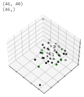
6. Results

My dataset consists of three features, 46 sample s in total, and 40 dimensional features  

 

It can be seen from the results that the dimensionality reduction effect of PCA is not obvious!

7. TSNE dimensionality reduction

Then the dimension reduction method of tsne is tried

In fact, it is here:

pca = decomposition.PCA(n_components=3)
pca.fit(x_data)
X = pca.transform(x_data) #Drop to 3D
#print(X)

Replaced with:

pca_tsne = TSNE(n_components=3)  
X = pca_tsne.fit_transform(x_data)  
#print(X)

The final result is:

The effect is not very good

Because the results from the previous model show that the accuracy of label 0 is very high, we try to see that the classification effect of label 0 is very good, that is, it is relatively concentrated, but the dimension reduction results can not get this conclusion. So the little teacher asked me not to use the dimensionality reduction data, but to try with the original data, and train with LR linear model on the original data to see how the effect is. But I don't know yet. I checked the application example of LR, which is classified into three categories. I can only process data with two-dimensional characteristics, while my data is 40 dimensional. I don't know how to change wuwuwuwuwuwuwuwuwuwuwuwuwuwuwuwuwuwuwuwuwuwuwuwuwuwuwuwuwuwuwuwuwuwuwuwuwuwuwuwuwuwuwuwuwuwuwuwuwuwuwuwuwuwuwuwuwuwu~