SAR (Simple Algorithm for Recommendation) is a fast and scalable adaptive algorithm, which can provide personalized recommendations according to users' transaction history The essence of SAR is nearest neighbor collaborative filtering It promotes by understanding the similarity between projects, and recommends similar projects to users with existing affinity

SAR is a fast scalable adaptive algorithm for personalized recommendations based on user transaction history   and items description. The core idea behind SAR is to recommend items like those that a user already has  demonstrated an affinity to. It does this by 
1) estimating the affinity of users for items,
2) estimating  similarity across items, and then 
3) combining the estimates to generate a set of recommendations for a given user.

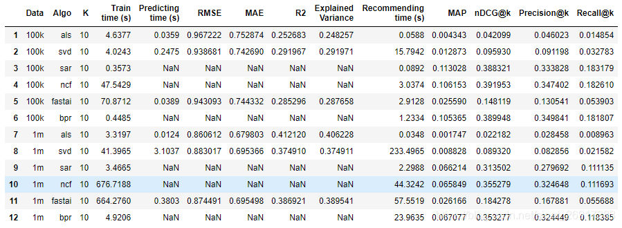
Effect of SAR model:

ALS can refer to: Exercise ｜ implementation of python collaborative filtering ALS model: commodity recommendation + user population amplification

Article catalog

• 1 model principle
• • 1.1 SAR calculation flow chart
  • 1.2 co occurrence matrix
  • 1.3 item similarity matrix
  • 1.4 user affinity score - affinity matrix
  • 1.5 additional features of SAR
• 2 case 1: use of simple SAR
• • 2.1 appearance of data set
  • 2.2 split of training / verification set
  • 2.3 SAR model initialization
  • 2.4 training and prediction
  • 2.5 evaluation
  • 2.6 independent forecast
• 3 SAR properties
• • 3.1 * * some basic attributes:**
  • 3.2 **item occurrence frequency**
  • 3.3 co occurrence matrix C of * * item-2-item**
  • 3.4 **affinity user item correlation matrix A**
  • 3.5 **affinity user item correlation matrix A - Standardization**
  • 3.6 recommendation score matrix - R matrix
• 4 case 2: deep dive SAR use
• • 4.1 Load data + Split the data
  • 4.2 SAR initialization
  • 4.3 model training + prediction
  • 4.4 evaluation
• reference

1 model principle

1.1 SAR calculation flow chart

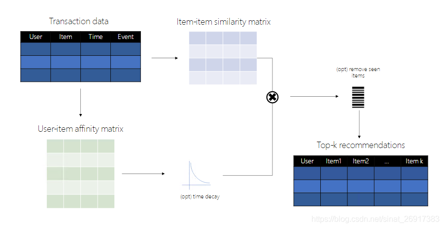
SAR calculation steps:

• C matrix, co occurrence matrix. First calculate the co-occurrence probability matrix of item to item. The value of the matrix represents the freq of two items appearing in the same user at the same time
• S matrix, item similarity matrix (based on item co-occurrence probability matrix) for Standardization (based on jaccard similarity, equivalent to a weighted average of i2i, primary compression / scaling of C matrix)
• A matrix, affinity matrix, user item incidence matrix (through ranking or reading, rating or viewing)
• S matrix * A matrix = R, recommendation score matrix
• Intercept everyone's top-k results

1.2 co occurrence matrix

SAR defines similarity based on item - to - item co - occurrence data Co - occurrence is defined as the number of times two items appear together for a given user We can express the co-occurrence of all items as m\times m (representing the number of items) Co occurrence matrix C has the following characteristics:

• Symmetrical, so c_{i,j} = c_{j,i}
• Nonnegative: c_{i,j} \geq 0
• Events are at least as large as those that occur simultaneously. That is, the largest element of each row (and column) is located on the main diagonal: \ forall(i,j) C_{i,i},C_{j,j} \geq C_{i,j} .

1.3 item similarity matrix

S matrix = primary compression / scaling of C matrix Once we have a co-occurrence matrix, we can obtain the project similarity matrix by rescaling co-occurrence according to a given metric: Jaccard, lift, and counts. If c_{ii} and c_{jj} is the ith and jth diagonal elements of matrix C, then the rescale option is:

• Jaccard: s_{ij}=\frac{c_{ij}}{(c_{ii}+c_{jj}-c_{ij})}
• lift: s_{ij}=\frac{c_{ij}}{(c_{ii} \times c_{jj})}
• counts: s_{ij}=c_{ij}

Usually, use counts as a similarity measure is conducive to predictability, which means that the most popular items are recommended most of the time. On the contrary lift is conducive to discovery / accidental discovery: a project that is not very popular but generally favored by a small number of users is more likely to be recommended Jaccard is a compromise between the two

1.4 user affinity score - affinity matrix

The affinity matrix in SAR captures the strength of the relationship between each user and the items with which the user has interacted. SAR contains two factors that may affect user affinity:

It can consider information about the type of user item interaction through different weights of different events (for example, it can weigh events in which the user rated a specific item more heavily than the events in which the user viewed the item) When a user item event occurs, it can consider information about the (for example, it can discount the value of events that occurred in the distant past) Formalize these factors to provide us with the expression of user item affinity: a_{ij}=\sum_k w_k \left(\frac{1}{2}\right)^{\frac{t_0-t_k}{T}}

• Affinity a{uj} represents the ith user and the jth item, and is the weighted sum of all k events (including the ith user and the jth item).
• w_k represents the weight of a specific event, and the power of the two terms reflects the event of temporary discount
• (\ frac{1}{2})^n scale factor causes parameter T as half-life: event T units before t_0 will be given half the weight as those that occur at t_0
• Repeating this calculation for all n users and m items will produce n\times m matrix A A simplification of the above expression can be obtained by setting all weights equal to 1 (valid ignore event types), or by setting the half-life parameter T to infinity (ignore transaction time)

1.5 additional features of SAR

Advantages of SAR:

• High precision, easy to train and deploy algorithms
• Fast training requires only simple counting to construct a matrix for predicting time.
• Fast scoring only involves the multiplication of similarity matrix and affinity vector

Disadvantages:

• There is no use of side information, so it is a big problem. There are no user attributes and item attributes
• A matrix of m*m will be formed. M is the number of item s, which will eat memory
• SAR supports implicit rating schemes, but it does not predict ratings
• Incremental training is not available for the time being, and only known can be predicted. If a new user / item is selected, it will be difficult to push

Additional function points:

• During prediction, the items in the training set can be removed. The significance is that it is not recommended to browse the items previously by the user again. See model.recommend_k_items(test, remove_seen=True) - (flag to remove items seen in training from recommendation)
• In terms of time decay half-life, the longer the time, the less attention will be paid to it

2 case 1: use of simple SAR

The lengthy code will not be described in detail. See the following for details: sar_movielens.ipynb , only the core ones here.

2.1 appearance of data set

data = movielens.load_pandas_df(
    size=MOVIELENS_DATA_SIZE
)

# Convert the float precision to 32-bit in order to reduce memory consumption 
data['rating'] = data['rating'].astype(np.float32)

data.head()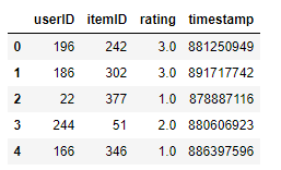

The basic elements are as follows: < user >, < item >, < score >, < time >, and the format is mainly pandas

2.2 split of training / verification set

train, test = python_stratified_split(data, ratio=0.75, col_user='userID', col_item='itemID', seed=42)

Since SAR generation recommendations are based on user preferences, all users in test settings must also exist in the training set. For this case, we can use the python_trained_split function provided to stretch out a percentage (25% in this case) from each user's items, but ensure that all users are training and testing the data set.

All users need to be in the system, so when splitting the training set and test set, ensure that everyone is there. Then someone may have 10 behaviors, and x times are extracted as the test set and 10-x as the training set

The splitting function is:

python_stratified_split(
    data,
    ratio=0.75,
    min_rating=1,
    filter_by='user',
    col_user='userID',
    col_item='itemID',
    seed=42,
)

    """Pandas stratified splitter.
    
    For each user / item, the split function takes proportions of ratings which is
    specified by the split ratio(s). The split is stratified.

    Args:
        data (pd.DataFrame): Pandas DataFrame to be split.
        ratio (float or list): Ratio for splitting data. If it is a single float number
            it splits data into two halves and the ratio argument indicates the ratio of
            training data set; if it is a list of float numbers, the splitter splits
            data into several portions corresponding to the split ratios. If a list is
            provided and the ratios are not summed to 1, they will be normalized.
        seed (int): Seed.
        min_rating (int): minimum number of ratings for user or item.
        filter_by (str): either "user" or "item", depending on which of the two is to
            filter with min_rating.
        col_user (str): column name of user IDs.
        col_item (str): column name of item IDs.

    Returns:
        list: Splits of the input data as pd.DataFrame.
    """

Among them, min_rating=1 minimum rating is used as the threshold.

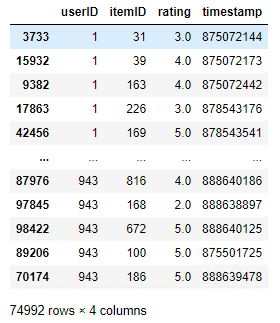
train dataset:

2.3 SAR model initialization

Example:

logging.basicConfig(level=logging.DEBUG, 
                    format='%(asctime)s %(levelname)-8s %(message)s')

model = SAR(
    col_user="userID",
    col_item="itemID",
    col_rating="rating",
    col_timestamp="timestamp",
    similarity_type="jaccard", 
    time_decay_coefficient=30, 
    timedecay_formula=True,
    normalize=True
)

SAR function initialization:

SAR(
    col_user='userID',
    col_item='itemID',
    col_rating='rating',
    col_timestamp='timestamp',
    col_prediction='prediction',
    similarity_type='jaccard',
    time_decay_coefficient=30,
    time_now=None,
    timedecay_formula=False,
    threshold=1,
    normalize=False,
)

English Interpretation:

Args:
     col_user (str): user column name
     col_item (str): item column name
     col_rating (str): rating column name
     col_timestamp (str): timestamp column name
     col_prediction (str): prediction column name
     similarity_type (str): ['cooccurrence', 'jaccard', 'lift'] option for computing item-item similarity
     time_decay_coefficient (float): number of days till ratings are decayed by 1/2
     time_now (int | None): current time for time decay calculation
     timedecay_formula (bool): flag to apply time decay
     threshold (int): item-item co-occurrences below this threshold will be removed
     normalize (bool): option for normalizing predictions to scale of original ratings

These include:

• similarity_type, from the stage of C matrix - > s matrix, similar function type, similarity_ There are three types: Options for the metric include Jaccard, lift, and counts
• col_timestamp, time decay
• time_ decay_ Coefficent, time attenuation parameter
• time_now, current time, confirm time attenuation
• threshold, co-occurrence of C matrix, low frequency removal
• normalize, is affinity matrix A standardized

2.4 training and prediction

Training code:

with Timer() as train_time:
    model.fit(train)

print("Took {} seconds for training.".format(train_time.interval))

Overall dataset forecast:

with Timer() as test_time:
    top_k = model.recommend_k_items(test, remove_seen=True)

print("Took {} seconds for prediction.".format(test_time.interval))

The test format is the same as the train format:

At this time, recommend is predicted_ k_ Items are expressed as:

model.recommend_k_items(test, top_k=10, sort_top_k=True, remove_seen=False)

Args:
    test (pd.DataFrame): users to test,pandas that will do
    top_k (int): number of top items to recommend,top items Ranking of
    sort_top_k (bool): flag to sort top k results,Sort
    remove_seen (bool): flag to remove items seen in training from recommendation,Remove recommended from training item,Extend some that have not been recommended before

Returns:
    pd.DataFrame: top k recommendation items for each user

Several of them, remove_ See is to remove the items recommended in the training and extend some items that have not been recommended before. The applicable scenario is to recommend content you haven't seen before.

2.5 evaluation

According to reco_ Python in utils_ The evaluate module provides several common ranking indicators to evaluate the performance of SAR. We will consider the average accuracy (MAP), normalized Cumulative Return (NDCG), accuracy and recall of the first k products per user calculated by SAR. Each evaluation method specifies the user, product, and rating column names.

eval_map = map_at_k(test, top_k, col_user='userID', col_item='itemID', col_rating='rating', k=TOP_K)
eval_ndcg = ndcg_at_k(test, top_k, col_user='userID', col_item='itemID', col_rating='rating', k=TOP_K)
eval_precision = precision_at_k(test, top_k, col_user='userID', col_item='itemID', col_rating='rating', k=TOP_K)
...

2.6 independent forecast

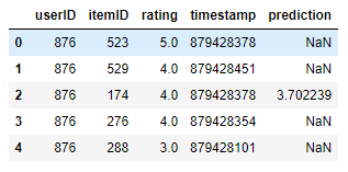
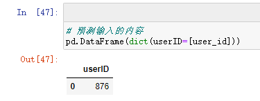
# Now let's look at the results for a specific user
user_id = 876

ground_truth = test[test['userID']==user_id].sort_values(by='rating', ascending=False)[:TOP_K]
prediction = model.recommend_k_items(pd.DataFrame(dict(userID=[user_id])), remove_seen=True) 
pd.merge(ground_truth, prediction, on=['userID', 'itemID'], how='left')

Of course, it is also possible here. Batch output: model. Recommended_ k_ items(pd.DataFrame(dict(userID=[user_id1,user_id2]))

Output:

Enter a special user number and output the corresponding content

Here, the test data style is:

From the above, we can see that the highest rated items in the test set recommended by the model top-k are adjusted, while other items remain unchanged. The offline evaluation algorithm is very difficult, because the test set only contains historical records and cannot represent the user's actual preference in the range of all items. For this problem, we can also use other algorithms (1) Or use hyper parameters (2) for optimization.

In practical applications, most of them are hybrid integrated recommendation systems, such as UserCF + ItemCF, ItemCF + Content-based or some other unique optimization methods. This part is described in detail in Aggarwal's recommendation system. Hyper parameters: it is the concept of machine learning (ML). In ml, the parameters that have been set are called According to my personal understanding, what the original text wants to say here is to continuously optimize the model through machine learning on incremental data.

3 SAR properties

Two official examples:

from reco_utils.recommender.sar import SAR
from reco_utils.recommender.sar.sar_singlenode import SARSingleNode

Both are the same program: from. Sar_singlenode import sarsinglenode as SAR

See the following for specific attributes: sar_singlenode.py

3.1 some basic attributes:

# Number of model item; number of user
len(model.item2index),model.user2index

# Number of items
model.n_items

# Number of people in the model
model.n_users

# Highest score
model.rating_max

# Lowest score
model.rating_min

# Similarity type: jaccard - initializes the generation of correlation matrix 'affinity matrix' in SAR
model.similarity_type

3.2 frequency of item occurrence

model.item_frequencies 
# array([126.,  69.,  66., ...,   1.,   1.,   1.])

3.3 co occurrence matrix C of item-2-item

# Similarity between model item items
# (1649, 1649)
model.item_similarity

3.4 affinity user item correlation matrix A

# General affinity matrix (943, 1649)
# U is the user_affinity matrix The co-occurrence matrix is defined as :math:`C = U^T * U`
model.user_affinity.todense()

This matrix is relatively large and sparse. Specific usage: Use of scipy.sparse, pandas.sparse and sklearn sparse matrices

3.5 affinity user item correlation matrix A - Standardization

# General affinity matrix (943, 1649)
# U is the user_affinity matrix The co-occurrence matrix is defined as :math:`C = U^T * U`
model.normalize # Is True standardized
model.unity_user_affinity.todense()

This matrix is relatively large and sparse. Specific usage: Use of scipy.sparse, pandas.sparse and sklearn sparse matrices

3.6 recommendation score matrix - R matrix

There is no R matrix here, Requires S matrix * A matrix = R, recommendation score matrix

4 case 2: deep dive SAR use

The lengthy code will not be described in detail. See the following for details: sar_deep_dive.ipynb , only the core ones here.

4.1 Load data + Split the data

data = movielens.load_pandas_df(
    size=MOVIELENS_DATA_SIZE,
    header=['UserId', 'MovieId', 'Rating', 'Timestamp'],
    title_col='Title'
)

# Convert the float precision to 32-bit in order to reduce memory consumption 
data.loc[:, 'Rating'] = data['Rating'].astype(np.float32)

data.head()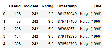

Segmentation data:

train, test = python_stratified_split(data, ratio=0.75, col_user=header["col_user"], col_item=header["col_item"], seed=42)

4.2 SAR initialization

# set log level to INFO
logging.basicConfig(level=logging.DEBUG, 
                    format='%(asctime)s %(levelname)-8s %(message)s')

header = {
    "col_user": "UserId",
    "col_item": "MovieId",
    "col_rating": "Rating",
    "col_timestamp": "Timestamp",
    "col_prediction": "Prediction",
}
model = SARSingleNode(
    similarity_type="jaccard", 
    time_decay_coefficient=30, 
    time_now=None, 
    timedecay_formula=True, 
    **header
)

Similar to the previous case initialization, the main attributes are:

SARSingleNode(
    col_user='userID',
    col_item='itemID',
    col_rating='rating',
    col_timestamp='timestamp',
    col_prediction='prediction',
    similarity_type='jaccard',
    time_decay_coefficient=30,
    time_now=None,
    timedecay_formula=False,
    threshold=1,
    normalize=False,
)

In this case, for the illustration purpose, the following parameter values are used:

T show in the formula of section 1.2) time_nownone, time reason reference.timereason_formulatruewhere time reason formula is used

4.3 model training + prediction

# train
model.fit(train)
# forecast
top_k = model.recommend_k_items(test, remove_seen=True)
# Exhibition
top_k_with_titles = (top_k.join(data[['MovieId', 'Title']].drop_duplicates().set_index('MovieId'), 
                                on='MovieId', 
                                how='inner').sort_values(by=['UserId', 'Prediction'], ascending=False))
display(top_k_with_titles.head(10))

4.4 evaluation

# all ranking metrics have the same arguments
args = [test, top_k]
kwargs = dict(col_user='UserId', 
              col_item='MovieId', 
              col_rating='Rating', 
              col_prediction='Prediction', 
              relevancy_method='top_k', 
              k=TOP_K)

eval_map = map_at_k(*args, **kwargs)
eval_ndcg = ndcg_at_k(*args, **kwargs)
eval_precision = precision_at_k(*args, **kwargs)
eval_recall = recall_at_k(*args, **kwargs)

The calculated indicators are as follows:

Model:
Top K:		 10
MAP:		 0.095544
NDCG:		 0.350232
Precision@K:	 0.305726
Recall@K:	 0.164690

reference

1 Recommended system SAR model 2 sar_movielens.ipynb 3 sar_deep_dive.ipynb 4. The core code is: sar_singlenode.py 5 Microsoft SAR - recommended system practice notes