Common method

Using neural network: (neural network of CIFAR10)

You can see that the input data is a picture of 3 channels 3232.
After 55 convolution kernel, 323232 data are obtained.
When defining a convolution layer, look at how much padding is.

You can find the formula on the official website:

Obviously, H is 32, division defaults to 1, and kernel_size= 5，
So only stripe and padding don't know this formula.
Suppose that stripe is 1, then padding is 2,
If you assume that stripe is 2, padding is 10 +, which is obviously unreasonable.
So at this time, it is calculated that stripe is 1 and padding is 2. The default string of the parameter is
1. No setting.

Then the convolution layer is set to self conv1 = Conv2d(3, 32, 5, padding=2)
Then comes the setting of the maximum pool layer: self maxpool1 = MaxPool2d(2)

By analogy, define the whole convolution and pooling network above. Don't forget that there are two linear layers at the end.

		self.conv1 = Conv2d(3, 32, 5, padding=2)
        self.maxpool1 = MaxPool2d(2)

        self.conv2 = Conv2d(32,32,5,padding=2)
        self.maxpool2 = MaxPool2d(2)

        self.conv3 = Conv2d(32,64,5,padding=2)
        self.maxpool3 = MaxPool2d(2)
        
        # Linear layer
  		self.flatten = Flatten() # Expand the data into one dimension
        self.linear1 = Linear(1024,64) # Why is this 1024? I'll explain later
        self.linear2 = Linear(64,10)

Then directly let the data pass through these layers one by one in foreword.

def forward(self,x):
        x = self.conv1(x)
        x = self.maxpool1(x)
        x = self.conv2(x)
        x = self.maxpool2(x)
        x = self.conv3(x)
        x = self.maxpool3(x)
        x = self.linear1(x)
        x = self.linear2(x)
        return x

Join the data to verify the correctness of the network:

text = Text()
inputs = torch.ones((64, 3, 32, 32))
output = text(inputs)
print(output.shape)

You can see the output torch Size([64, 10])

After convolution and pooling, the last linear layer needs to know the input data dimension, so you can look at the data dimension before writing the linear layer, torch Size([64, 64, 4, 4]) . After flattening him, it is obviously [6444]
Therefore, we know that the dimension entering the linear layer is [64 * 1024].
Torch can be obtained directly by using the flatten() function Size([64, 1024]).

Full code:

import torch
from torch import nn
from torch.nn import Conv2d, MaxPool2d, Flatten, Linear


class Text(nn.Module):
    def __init__(self):
        super(Text, self).__init__()
        self.conv1 = Conv2d(3, 32, 5, padding=2)
        self.maxpool1 = MaxPool2d(2)

        self.conv2 = Conv2d(32, 32, 5, padding=2)
        self.maxpool2 = MaxPool2d(2)

        self.conv3 = Conv2d(32, 64, 5, padding=2)
        self.maxpool3 = MaxPool2d(2)
        # Linear layer
        self.flatten = Flatten()  # Expand the data into one dimension
        self.linear1 = Linear(1024, 64)
        self.linear2 = Linear(64, 10)

    def forward(self, x):
        x = self.conv1(x)
        x = self.maxpool1(x)
        x = self.conv2(x)
        x = self.maxpool2(x)
        x = self.conv3(x)
        x = self.maxpool3(x)
        x = self.flatten(x)
        x = self.linear1(x)
        x = self.linear2(x)
        return x


text = Text()
inputs = torch.ones((64, 3, 32, 32))
output = text(inputs)
print(output.shape)

sequential method

The code after sequential rewriting simplifies the steps of writing layer by layer above. You can understand it at a glance

import torch
from torch import nn
from torch.nn import Conv2d, MaxPool2d, Flatten, Linear, Sequential

class Text(nn.Module):
    def __init__(self):
        super(Text, self).__init__()
        self.model1 = Sequential(
            Conv2d(3, 32, 5, padding=2),
            MaxPool2d(2),

            Conv2d(32, 32, 5, padding=2),
            MaxPool2d(2),

            Conv2d(32, 64, 5, padding=2),
            MaxPool2d(2),
            # Linear layer
            Flatten(),  # Expand the data into one dimension
            Linear(1024, 64),
            Linear(64, 10),

        )

    def forward(self, x):
        x = self.model1
        return x

text = Text()
inputs = torch.ones((64, 3, 32, 32))
output = text(inputs)
print(output.shape)

Use tansorbboard to visualize various data in the convolution layer

Add three lines of code to visualize the various layers above.

write = SummaryWriter('logs')
write.add_graph(text,inputs)
write.close()

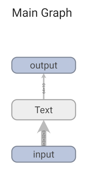
like this:

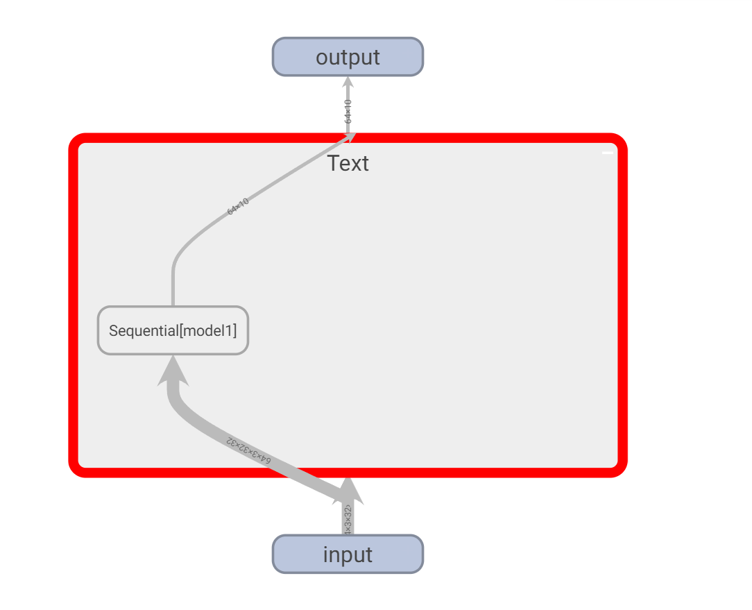
Each of them can be opened. Double click the icon to zoom in. For example, I double-click Text.

Double click the model we created:
You can see that there are various layers we have established here.

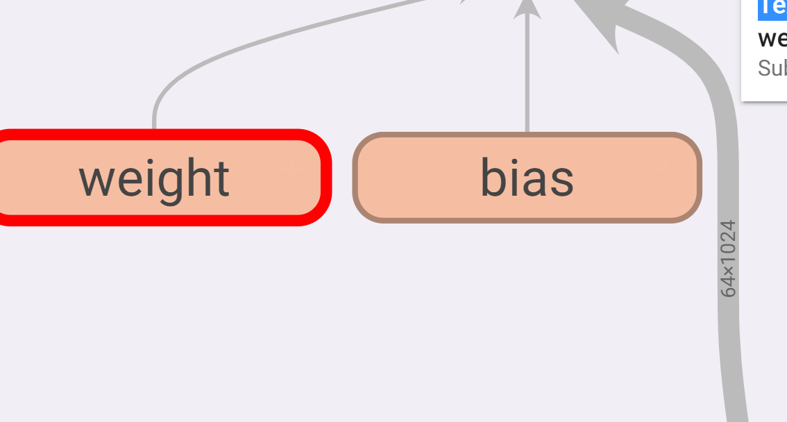
You can continue to double-click to zoom in:
You can see all kinds of data inside. For example, the input and output data dimensions in the gray channel on the right bring great convenience to the later debugging of the model.