Datawhale - (scikit learn tutorial) - task01 (linear regression and logistic regression) - 202112

Link to scikit learn tutorial for DataWhale
1, Linear regression
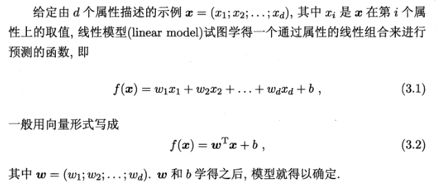
​​1. Basic form of linear regression

2. Gradient descent training

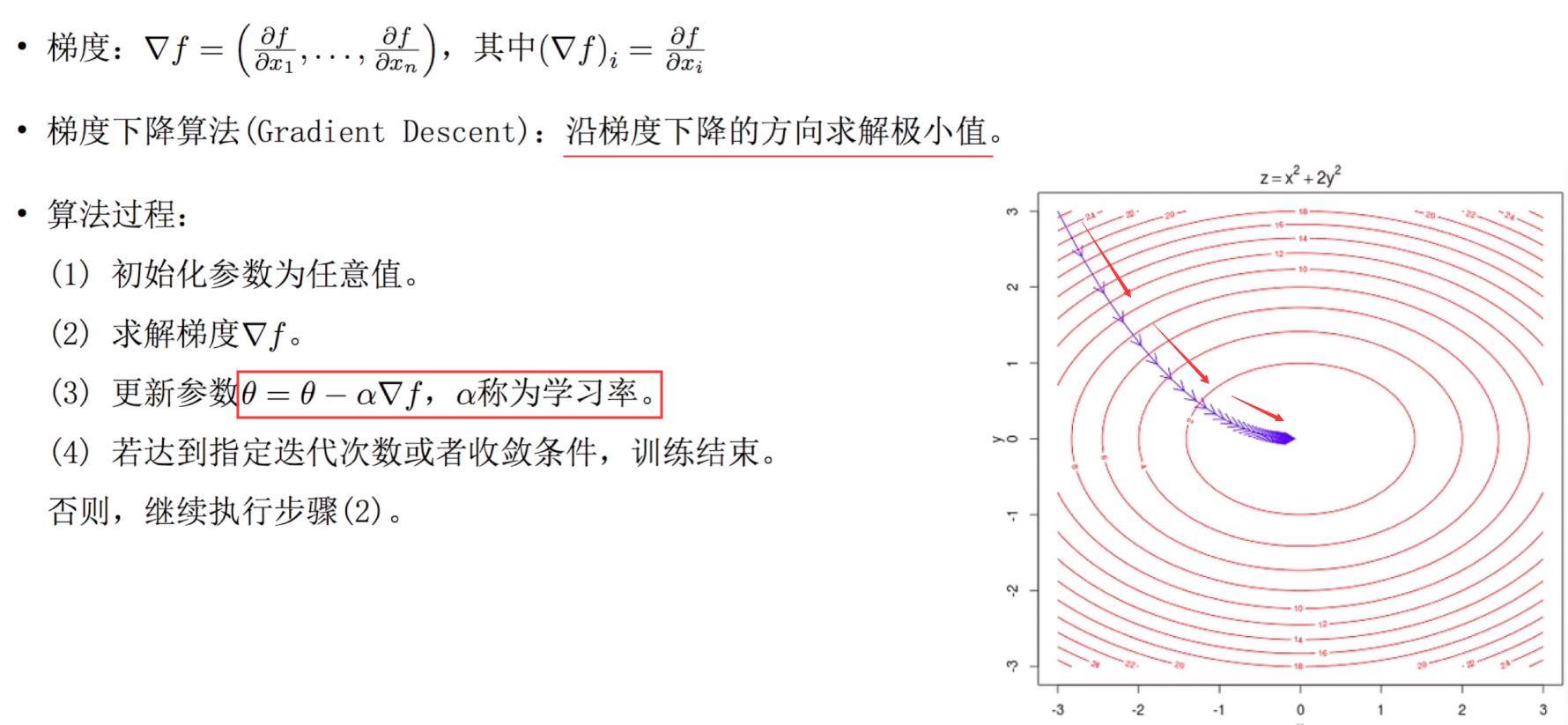
Assuming a given model h ( θ ) = ∑ j = 0 n θ j x j h(\theta)=\sum_{j=0}^{n} \theta_{j} x_{j} h( θ)= ∑j=0n​ θ J ， xj ， and objective function (loss function): J ( θ ) = 1 m ∑ i = 0 m ( h θ ( x i ) − y i ) 2 J(\theta)=\frac{1}{m} \sum_{i=0}^{m}\left(h_{\theta}\left(x^{i}\right)-y^{i}\right)^{2} J( θ)= m1​∑i=0m​(h θ (xi) − yi)2, where m m m represents the amount of data. Our goal is to J ( θ ) J(\theta) J( θ) As small as possible, so add here 1 2 \frac{1}{2} 21. For the following simplification, i.e J ( θ ) = 1 2 m ∑ i = 0 m ( y i − h θ ( x i ) ) 2 J(\theta)=\frac{1}{2m} \sum_{i=0}^{m}\left(y^{i}-h_{\theta}\left(x^{i}\right)\right)^{2} J(θ)=2m1​∑i=0m​(yi−hθ​(xi))2.
Then the gradient is:
∂ J ( θ ) ∂ θ j = 1 m ∑ i = 0 m ( y i − h θ ( x i ) ) ∂ ∂ θ j ( y i − h θ ( x i ) ) = − 1 m ∑ i = 0 m ( y i − h θ ( x i ) ) ∂ ∂ θ j ( ∑ j = 0 n θ j x j i − y i ) = − 1 m ∑ i = 0 m ( y i − h θ ( x i ) ) x j i = 1 m ∑ i = 0 m ( h θ ( x i ) − y i ) ) x j i \begin{aligned} \frac{\partial J(\theta)}{\partial \theta_{j}} &=\frac{1}{m} \sum_{i=0}^{m}\left(y^{i}-h_{\theta}\left(x^{i}\right)\right) \frac{\partial}{\partial \theta_{j}}\left(y^{i}-h_{\theta}\left(x^{i}\right)\right) \\ &=-\frac{1}{m} \sum_{i=0}^{m}\left(y^{i}-h_{\theta}\left(x^{i}\right)\right) \frac{\partial}{\partial \theta_{j}}\left(\sum_{j=0}^{n} \theta_{j} x_{j}^{i}-y^{i}\right) \\ &=-\frac{1}{m} \sum_{i=0}^{m}\left(y^{i}-h_{\theta}\left(x^{i}\right)\right) x_{j}^{i}\\ &=\frac{1}{m} \sum_{i=0}^{m}\left(h_{\theta}(x^{i})-y^{i})\right) x_{j}^{i} \end{aligned} ∂θj​∂J(θ)​​=m1​i=0∑m​(yi−hθ​(xi))∂θj​∂​(yi−hθ​(xi))=−m1​i=0∑m​(yi−hθ​(xi))∂θj​∂​(j=0∑n​θj​xji​−yi)=−m1​i=0∑m​(yi−hθ​(xi))xji​=m1​i=0∑m​(hθ​(xi)−yi))xji​​

set up x x x is a matrix of (m,n) dimensions, y y y is the matrix of (m,1) dimension, h θ h_{\theta} h θ Is the predicted value, dimension and y y y is the same, then the gradient is represented by a matrix as follows:
∂ J ( θ ) ∂ θ j = 1 m x T ( h θ − y ) \frac{\partial J(\theta)}{\partial \theta_{j}} = \frac{1}{m}x^{T}(h_{\theta}-y) ∂θj​∂J(θ)​=m1​xT(hθ​−y)

3. Implementation of univariate linear regression code
(1) numpy is implemented using gradient descent

import numpy as np
import matplotlib.pyplot as plt

def true_fun(X):
    return 1.5*X + 0.2

np.random.seed(0) # Random seed
n_samples = 30
'''Generate random data as training set'''
X_train = np.sort(np.random.rand(n_samples)) 
y_train = (true_fun(X_train) + np.random.randn(n_samples) * 0.05).reshape(n_samples,1)
data_X = []
for x in X_train:
    data_X.append([1,x])
data_X = np.array((data_X))

m,p = np.shape(data_X) # m. Data volume p: number of features
max_iter = 1000 # Iterated algebra
weights = np.ones((p,1))  
alpha = 0.1 # Learning rate
for i in range(0,max_iter):
    error = np.dot(data_X,weights)- y_train
    gradient = data_X.transpose().dot(error)/m
    weights = weights - alpha * gradient
print("Output parameters w:",weights[1:][0]) # Output model parameter w
print("Output parameters:b",weights[0]) # Output parameter b

X_test = np.linspace(0, 1, 100)
plt.plot(X_test, X_test*weights[1][0]+weights[0][0], label="Model") 
plt.plot(X_test, true_fun(X_test), label="True function")
plt.scatter(X_train,y_train) # Draw the points of the training set
plt.legend(loc="best")
plt.show()

(2) sklearn to realize univariate linear regression

import numpy as np
from sklearn.linear_model import LinearRegression # Import linear regression model
import matplotlib.pyplot as plt

def true_fun(X):
    return 1.5*X + 0.2

np.random.seed(0) # Random seed
n_samples = 30
'''Generate random data as training set'''
X_train = np.sort(np.random.rand(n_samples)) 
y_train = (true_fun(X_train) + np.random.randn(n_samples) * 0.05).reshape(n_samples,1)

model = LinearRegression() # Define model
model.fit(X_train[:,np.newaxis], y_train) # Training model

print("Output parameters w:",model.coef_) # Output model parameter w
print("Output parameters:b",model.intercept_) # Output parameter b

X_test = np.linspace(0, 1, 100)
plt.plot(X_test, model.predict(X_test[:, np.newaxis]), label="Model")
plt.plot(X_test, true_fun(X_test), label="True function")
plt.scatter(X_train,y_train) # Draw the points of the training set
plt.legend(loc="best")
plt.show()

(3) sklearn to realize multiple linear regression

from sklearn.linear_model import LinearRegression

X_train = [[1,1,1],[1,1,2],[1,2,1]]
y_train = [[6],[9],[8]]
 
model = LinearRegression()
model.fit(X_train, y_train)
print("Output parameters w:",model.coef_) # Output parameters w1,w2,w3
print("Output parameters b:",model.intercept_) # Output parameter b
test_X = [[1,3,5]]
pred_y = model.predict(test_X)
print("Prediction results:",pred_y)

2, Polynomial regression and over fitting and under fitting

1. Training set
   The data set used to train the parameters in the model
2. Validation set
   It is used to test the state and convergence of the model in the training process. It is usually used to adjust the super parameters. According to the performance of several groups of model verification sets, it determines which group of super parameters has the best performance. At the same time, the validation set can also be used to monitor whether the model has been fitted during the training process. Generally speaking, after the performance of the validation set is stable, if you continue training, the performance of the training set will continue to rise, but the validation set will not rise but fall, so over fitting generally occurs. Therefore, the verification set is also used to judge when to stop training.
3. Test set
   The test set is used to evaluate the generalization ability of the model, that is, the training set is used to adjust the parameters. Before, the model uses the verification set to determine the super parameters, and finally uses a different data set to check the model.
4. Cross validation
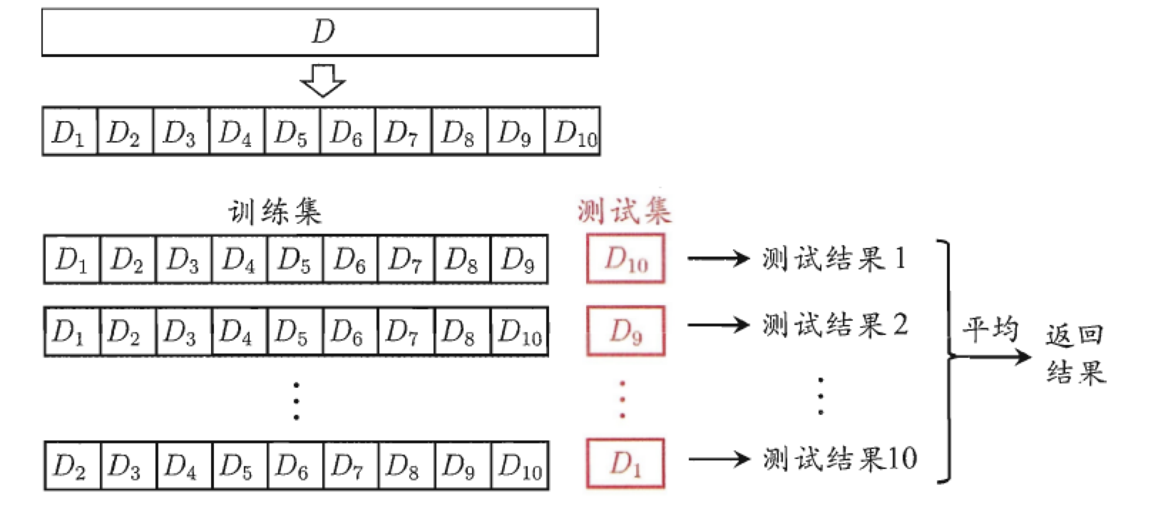
   The function of cross validation method is to try to use different training set / test set division to do multiple groups of different training / tests on the model, so as to deal with the problems of too one-sided test results and insufficient training data.
   
5. sklearn implementation of polynomial regression

import numpy as np
import matplotlib.pyplot as plt
from sklearn.pipeline import Pipeline
from sklearn.preprocessing import PolynomialFeatures
from sklearn.linear_model import LinearRegression
from sklearn.model_selection import cross_val_score

def true_fun(X):
    return np.cos(1.5 * np.pi * X)
np.random.seed(0)

n_samples = 30
degrees = [1, 4, 15] # Polynomial highest degree

X = np.sort(np.random.rand(n_samples)) 
y = true_fun(X) + np.random.randn(n_samples) * 0.1

plt.figure(figsize=(14, 5))
for i in range(len(degrees)):
    ax = plt.subplot(1, len(degrees), i + 1)
    plt.setp(ax, xticks=(), yticks=())

    polynomial_features = PolynomialFeatures(degree=degrees[i],
                                             include_bias=False)
    linear_regression = LinearRegression()
    pipeline = Pipeline([("polynomial_features", polynomial_features),
                         ("linear_regression", linear_regression)]) # Using pipline tandem model
    pipeline.fit(X[:, np.newaxis], y)

    # Use cross validation
    scores = cross_val_score(pipeline, X[:, np.newaxis], y,
                             scoring="neg_mean_squared_error", cv=10)
    X_test = np.linspace(0, 1, 100)
    plt.plot(X_test, pipeline.predict(X_test[:, np.newaxis]), label="Model")
    plt.plot(X_test, true_fun(X_test), label="True function")
    plt.scatter(X, y, edgecolor='b', s=20, label="Samples")
    plt.xlabel("x")
    plt.ylabel("y")
    plt.xlim((0, 1))
    plt.ylim((-2, 2))
    plt.legend(loc="best")
    plt.title("Degree {}\nMSE = {:.2e}(+/- {:.2e})".format(
        degrees[i], -scores.mean(), scores.std()))
plt.show()

2, Logistic regression

As with linear regression, we need to find n n n parameters:

z = θ 0 + θ 1 x + θ 2 x + . . . + θ n x = θ T x z=\theta_0+\theta_1x+\theta_2x+...+\theta_nx=\theta^Tx z=θ0​+θ1​x+θ2​x+...+θn​x=θTx

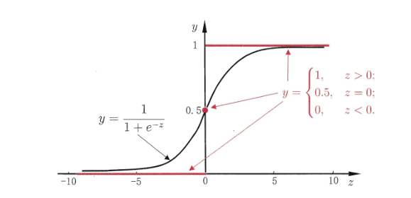
Logistic regression introduces nonlinear factors through Sigmoid function, which can easily deal with binary classification problems:

h θ ( x ) = g ( θ T x ) , g ( z ) = 1 1 + e − z h_{\theta}(x)=g\left(\theta^{T} x\right), g(z)=\frac{1}{1+e^{-z}} hθ​(x)=g(θTx),g(z)=1+e−z1​

Unlike linear regression, logistic regression uses the cross entropy loss function:

J ( θ ) = − 1 m [ ∑ i = 1 m ( y ( i ) log ⁡ h θ ( x ( i ) ) + ( 1 − y ( i ) ) log ⁡ ( 1 − h θ ( x ( i ) ) ) ] J(\theta)=-\frac{1}{m}\left[\sum_{i=1}^{m}\left(y^{(i)} \log h_{\theta}\left(x^{(i)}\right)+\left(1-y^{(i)}\right) \log \left(1-h_{\theta}\left(x^{(i)}\right)\right)\right]\right. J(θ)=−m1​[i=1∑m​(y(i)loghθ​(x(i))+(1−y(i))log(1−hθ​(x(i)))]

Its gradient is:

∂ J ( θ ) ∂ θ j = 1 m ∑ i = 0 m ( h θ − y i ( x i ) ) x j i \frac{\partial J(\theta)}{\partial \theta_{j}} = \frac{1}{m} \sum_{i=0}^{m}\left(h_{\theta}-y^{i}\left(x^{i}\right)\right) x_{j}^{i} ∂θj​∂J(θ)​=m1​i=0∑m​(hθ​−yi(xi))xji​

The form is the same as that of linear regression, but the hypothetical function is different. The logical regression is:
h θ ( x ) = 1 1 + e − θ T x h_{\theta}(x)=\frac{1}{1+e^{-\theta^{T} x}} hθ​(x)=1+e−θTx1​

The derivation is as follows:

∂ ∂ θ j J ( θ ) = ∂ ∂ θ j [ − 1 m ∑ i = 1 m [ y ( i ) log ⁡ ( h θ ( x ( i ) ) ) + ( 1 − y ( i ) ) log ⁡ ( 1 − h θ ( x ( i ) ) ) ] ] = − 1 m ∑ i = 1 m [ y ( i ) 1 h θ ( x ( i ) ) ) ∂ ∂ θ j h θ ( x ( i ) ) − ( 1 − y ( i ) ) 1 1 − h θ ( x ( i ) ) ∂ ∂ θ j h θ ( x ( i ) ) ] = − 1 m ∑ i = 1 m [ y ( i ) 1 h θ ( x ( i ) ) ) − ( 1 − y ( i ) ) 1 1 − h θ ( x ( i ) ) ] ∂ ∂ θ j h θ ( x ( i ) ) = − 1 m ∑ i = 1 m [ y ( i ) 1 h θ ( x ( i ) ) ) − ( 1 − y ( i ) ) 1 1 − h θ ( x ( i ) ) ] ∂ ∂ θ j g ( θ T x ( i ) ) \begin{aligned} \frac{\partial}{\partial \theta_{j}} J(\theta) &=\frac{\partial}{\partial \theta_{j}}\left[-\frac{1}{m} \sum_{i=1}^{m}\left[y^{(i)} \log \left(h_{\theta}\left(x^{(i)}\right)\right)+\left(1-y^{(i)}\right) \log \left(1-h_{\theta}\left(x^{(i)}\right)\right)\right]\right] \\ &=-\frac{1}{m} \sum_{i=1}^{m}\left[y^{(i)} \frac{1}{\left.h_{\theta}\left(x^{(i)}\right)\right)} \frac{\partial}{\partial \theta_{j}} h_{\theta}\left(x^{(i)}\right)-\left(1-y^{(i)}\right) \frac{1}{1-h_{\theta}\left(x^{(i)}\right)} \frac{\partial}{\partial \theta_{j}} h_{\theta}\left(x^{(i)}\right)\right] \\ &=-\frac{1}{m} \sum_{i=1}^{m}\left[y^{(i)} \frac{1}{\left.h_{\theta}\left(x^{(i)}\right)\right)}-\left(1-y^{(i)}\right) \frac{1}{1-h_{\theta}\left(x^{(i)}\right)}\right] \frac{\partial}{\partial \theta_{j}} h_{\theta}\left(x^{(i)}\right) \\ &=-\frac{1}{m} \sum_{i=1}^{m}\left[y^{(i)} \frac{1}{\left.h_{\theta}\left(x^{(i)}\right)\right)}-\left(1-y^{(i)}\right) \frac{1}{1-h_{\theta}\left(x^{(i)}\right)}\right] \frac{\partial}{\partial \theta_{j}} g\left(\theta^{T} x^{(i)}\right) \end{aligned} ∂θj​∂​J(θ)​=∂θj​∂​[−m1​i=1∑m​[y(i)log(hθ​(x(i)))+(1−y(i))log(1−hθ​(x(i)))]]=−m1​i=1∑m​[y(i)hθ​(x(i)))1​∂θj​∂​hθ​(x(i))−(1−y(i))1−hθ​(x(i))1​∂θj​∂​hθ​(x(i))]=−m1​i=1∑m​[y(i)hθ​(x(i)))1​−(1−y(i))1−hθ​(x(i))1​]∂θj​∂​hθ​(x(i))=−m1​i=1∑m​[y(i)hθ​(x(i)))1​−(1−y(i))1−hθ​(x(i))1​]∂θj​∂​g(θTx(i))​

Because:
∂ ∂ θ j g ( θ T x ( i ) ) = ∂ ∂ θ j 1 1 + e − θ T x ( i ) = e − θ T x ( i ) ( 1 + − θ T T x ( i ) ) 2 ∂ ∂ θ j θ T x ( i ) = g ( θ T x ( i ) ) ( 1 − g ( θ T x ( i ) ) ) x j ( i ) \begin{aligned} \frac{\partial}{\partial \theta_{j}} g\left(\theta^{T} x^{(i)}\right) &=\frac{\partial}{\partial \theta_{j}} \frac{1}{1+e^{-\theta^{T} x^{(i)}}} \\ &=\frac{e^{-\theta^{T} x^{(i)}}}{\left(1+^{-\theta} T^{T_{x}(i)}\right)^{2}} \frac{\partial}{\partial \theta_{j}} \theta^{T} x^{(i)} \\ &=g\left(\theta^{T} x^{(i)}\right)\left(1-g\left(\theta^{T} x^{(i)}\right)\right) x_{j}^{(i)} \end{aligned} ∂θj​∂​g(θTx(i))​=∂θj​∂​1+e−θTx(i)1​=(1+−θTTx​(i))2e−θTx(i)​∂θj​∂​θTx(i)=g(θTx(i))(1−g(θTx(i)))xj(i)​​
So:
∂ ∂ θ j J ( θ ) = − 1 m ∑ i = 1 m [ y ( i ) ( 1 − g ( θ T x ( i ) ) ) − ( 1 − y ( i ) ) g ( θ T x ( i ) ) ] x j ( i ) = − 1 m ∑ i = 1 m ( y ( i ) − g ( θ T x ( i ) ) ) x j ( i ) = 1 m ∑ i = 1 m ( h θ ( x ( i ) ) − y ( i ) ) x j ( i ) \begin{aligned} \frac{\partial}{\partial \theta_{j}} J(\theta) &=-\frac{1}{m} \sum_{i=1}^{m}\left[y^{(i)}\left(1-g\left(\theta^{T} x^{(i)}\right)\right)-\left(1-y^{(i)}\right) g\left(\theta^{T} x^{(i)}\right)\right] x_{j}^{(i)} \\ &=-\frac{1}{m} \sum_{i=1}^{m}\left(y^{(i)}-g\left(\theta^{T} x^{(i)}\right)\right) x_{j}^{(i)} \\ &=\frac{1}{m} \sum_{i=1}^{m}\left(h_{\theta}\left(x^{(i)}\right)-y^{(i)}\right) x_{j}^{(i)} \end{aligned} ∂θj​∂​J(θ)​=−m1​i=1∑m​[y(i)(1−g(θTx(i)))−(1−y(i))g(θTx(i))]xj(i)​=−m1​i=1∑m​(y(i)−g(θTx(i)))xj(i)​=m1​i=1∑m​(hθ​(x(i))−y(i))xj(i)​​

1. Logical regression is realized by numpy

import sys,os
curr_path = os.path.dirname(os.path.abspath(__file__)) # Absolute path of the current file
parent_path = os.path.dirname(curr_path) # Parent path
sys.path.append(parent_path) # Add path to system path

from Mnist.load_data import load_local_mnist

import numpy as np
import time


class LogisticRegression:
    def __init__(self, x_train, y_train, x_test, y_test):
        '''
        Args:
            x_train [Array]: Training set data
            y_train [Array]: Training set label
            x_test [Array]: Test set data
            y_test [Array]: Test set label
        '''
        self.x_train, self.y_train = x_train, y_train
        self.x_test, self.y_test = x_test, y_test
        # Convert the input data into matrix form to facilitate operation
        self.x_train_mat, self.x_test_mat = np.mat(
            self.x_train), np.mat(self.x_test)
        self.y_train_mat, self.y_test_mat = np.mat(
            self.y_test).T, np.mat(self.y_test).T
        # theta represents the parameters of the model, namely w and b
        self.theta = np.mat(np.zeros(len(x_train[0])))
        self.lr=0.001 # You can set learning rate optimization and use Adam and other optimizers
        self.n_iters=10  # Set the number of iterations
    @staticmethod
    def sigmoid(x):
        '''sigmoid function
        '''
        return 1.0/(1+np.exp(-x))
        
    def _predict(self,x_test_mat):
        P=self.sigmoid(np.dot(x_test_mat, self.theta.T))
        if P >= 0.5:
            return 1
        return 0
    def train(self):
        '''Training process, you can refer to pseudo code
        '''
        for i_iter in range(self.n_iters):
            for i in range(len(self.x_train)):
                result = self.sigmoid(np.dot(self.x_train_mat[i], self.theta.T))
                error = self.y_train[i]- result
                grad = error*self.x_train_mat[i]
                self.theta+= self.lr*grad
            print('LogisticRegression Model(learning_rate={},i_iter={})'.format(
            self.lr, i_iter+1))
    def save(self):
        '''Save model parameters to local file
        '''
        np.save(os.path.dirname(sys.argv[0])+"/theta.npy",self.theta)
    def load(self):
        self.theta=np.load(os.path.dirname(sys.argv[0])+"/theta.npy")
    def test(self):
         # Error value count
        error_count = 0
        #Verify each test sample in the test set
        for n in range(len(self.x_test)):
            y_predict=self._predict(self.x_test_mat[n])
            #If the mark is inconsistent with the prediction, the error value is increased by 1
            if self.y_test[n] != y_predict:
                error_count += 1
            print("accuracy=",1 - (error_count /(n+1)))
        #Return accuracy
        return 1 - error_count / len(self.x_test)

def normalized_dataset():
    # Load dataset, one_hot=False means that the output tag is in digital form, such as 3 instead of [0,0,0,1,0,0,0,0,0]
    (x_train, y_train), (x_test, y_test) = load_local_mnist(one_hot=False)
    # w and b are combined together, so the training data is increased by one dimension
    ones_col=[[1] for i in range(len(x_train))] # Generate a two-dimensional nested list of all 1, namely [[1], [1], [1]]
    x_train_modified=np.append(x_train,ones_col,axis=1)
    ones_col=[[1] for i in range(len(x_test))] # Generate a two-dimensional nested list of all 1, namely [[1], [1], [1]]
    x_test_modified=np.append(x_test,ones_col,axis=1)
    # Mnsit has 0-9 marks. Since it is a secondary classification task, it takes 0 as 1 and the rest as 0
    # It is verified that the accuracy is about 90% when < 5 is 1 > 5 is 0. It is speculated that after there are many numbers, the characteristics of different numbers may be chaotic, and a reasonable hyperplane cannot be calculated effectively
    # After checking the results of the previous perceptron, the accuracy rate is 81 when taking 5 as the boundary, and 98.91% when it is revised to 0 and the remainder
    # It seems that if the sample labels are miscellaneous, it does have a great impact on whether the hyperplane can be divided effectively
    y_train_modified=np.array([1 if y_train[i]==1 else 0 for i in range(len(y_train))])
    y_test_modified=np.array([1 if y_test[i]==1 else 0 for i in range(len(y_test))])
    return x_train_modified,y_train_modified,x_test_modified,y_test_modified

if __name__ == "__main__":
    start = time.time()   
    x_train_modified,y_train_modified,x_test_modified,y_test_modified = normalized_dataset()
    model=LogisticRegression(x_train_modified,y_train_modified,x_test_modified,y_test_modified)
    model.train()
    model.save()
    model.load()
    accur=model.test()
    end = time.time()
    print("total acc:",accur)
    print('time span:', end - start)

2. Logistic regression is realized by sklearn

import sys
from pathlib import Path
curr_path = str(Path().absolute())
parent_path = str(Path().absolute().parent)
sys.path.append(parent_path) # add current terminal path to sys.path

from Mnist.load_data import load_local_mnist

from sklearn.linear_model import LogisticRegression
from sklearn.metrics import classification_report

(X_train, y_train), (X_test, y_test) = load_local_mnist(normalize = False,one_hot = False)
model = LogisticRegression()
model.fit(X_train, y_train)
y_pred = model.predict(X_test)
print(classification_report(y_test, y_pred)) # Print report

import sys
from pathlib import Path
curr_path = str(Path().absolute())
parent_path = str(Path().absolute().parent)
sys.path.append(parent_path) # add current terminal path to sys.path

from Mnist.load_data import load_local_mnist

from sklearn.linear_model import LogisticRegression
from sklearn.metrics import classification_report

(X_train, y_train), (X_test, y_test) = load_local_mnist(normalize = False,one_hot = False)

X_train, y_train= X_train[:2000], y_train[:2000] 
X_test, y_test = X_test[:200],y_test[:200]

# solver: the optimizer used, lbfgs: Quasi Newton method, sag: random gradient descent
model = LogisticRegression(solver='lbfgs', max_iter=500) # lbfgs: Quasi Newton method
model.fit(X_train, y_train)
y_pred = model.predict(X_test)
print(classification_report(y_test, y_pred)) # Print report