Original link: http://tecdat.cn/?p=24721
In this paper, I use two examples that may be of interest to population ecologists to illustrate the use of "JAGS" to simulate data: the first is linear regression, and the second is to estimate animal survival rate (formulated as state space model).
Recently, I have been trying to simulate data from complex hierarchical models. I'm using JAGS now.
Simulation data JAGS is very convenient because you can use (almost) the same code for simulation and reasoning, and you can conduct simulation research (deviation, precision, interval) in the same environment (i.e. JAGS).
Linear regression example
Let's first load the packages required for this tutorial:
library(R2jags)
Then let's get straight to the point and let's generate data from the linear regression model. Use a data block and pass parameters as data.
data{
# Likelihood function:
for (i in 1:N){
y\[i\] ~  # tau is precision (1 / variance).

}
Here, alpha and beta are intercept and slope, precision or reciprocal of tau variance, y dependent variable and x explanatory variable.
We choose some values for the model parameters used as data:
# Simulated parameters
N  # sample
x <- 1:N # Predictor
alpha # intercept
beta  # Slope
sigma# Residual sd
 1/(sigma*sigma) # accuracy
# In the simulation step, the parameters are treated as data
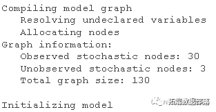
Now run JAGS; Please note that we monitor dependent variables instead of parameters, as we do in standard reasoning:
# Operation results
out
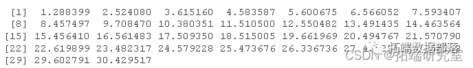
The output is a little messy and needs to be properly formatted:
# Reformat output
mcmc(out)
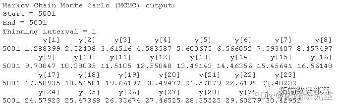
dim

dat
Now let's fit the model we used to simulate into the data we just generated. It is assumed that the reader is familiar with JAGS linear regression.
# Specifying models in BUGS language
model <-

for (i in 1:N){
y\[i\] ~ dnorm(mu\[i\], tau) # tau is precision (1 / variance)


alpha  intercept
beta # Slope
sigma  # standard deviation


# data
dta <- list(y = dt, N = length(at), x = x)

# Initial value
inits


# MCMC settings
ni <- 10000


# Calling JAGS from R
jags()
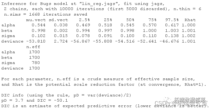
Let's look at the results and compare them with the parameters we used to simulate the data (see above):
# Summary posteriori
print(res)
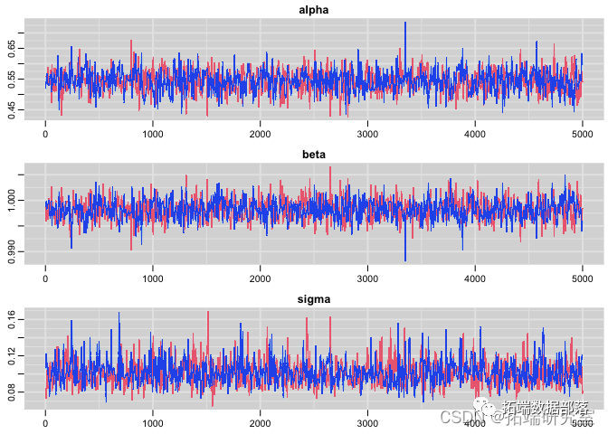
Check Convergence:
# Tracking chart
plot(res)
Plot the posterior distribution of regression parameters and residual standard deviation:
# Posterior distribution
plot(res)

Simulation example
I will now explain how to use JAGS to simulate data from models with constant survival and recapture probabilities. I assume that the reader is familiar with this model and its formula as a state space model.
Let's simulate it!
# Constant survival and recapture probability
for (i in 1:nd){
   for (t in f:(on-1)){

#probability
for (i in 1:nid){
   # Define latency and observations at first capture
   z\[i,f\[i\] <- 1
   mu2\[i,1\] <- 1 * z\[i,f\[i\] # It is detected as 1 at the first capture ("subject to the first capture").
   # Then deal with the future situation
   for (t in (f\[i\]+1):non){
      # Status process
      mu1\[i,t\] <- phi * z
      # Observation process
      mu2\[i,t\] <- p * z
Let's select some values for the parameters and store them in the data list:
# Parameters for simulation
n = 100 # Number of individuals
meanhi <- 0.8 # Survival rate
meap <- 0.6 # Recapture rate
data<-list
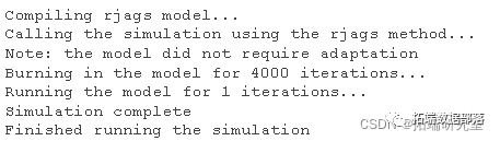
Now run JAGS:
out
Format output:
as.mcmc(out)

head(dat)
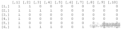
I only monitor the detection and non detection, but I can also obtain the simulation value of the state, that is, whether the individual is alive or dead in each case. You just need to modify the call to JAGS monitor=c("y","x") and modify the output accordingly.
Now we fit the Cormack jolly Seber (CJS) model to the data we just simulated, assuming that the parameters remain unchanged:
# Tendencies and constraints
for (i in 1:nd){
   for (t in f\[i\]:(nn-1)){


mehi ~ dunif(0, 1) # A priori value of mean survival
Me ~ dunif(0, 1) # A priori value of average recapture
# probability
for (i in 1:nd){
   # Defines the latency at the first capture
   z\[i\]\] <- 1
   for (t in (f\[i\]+1):nions){
      # State process
      z\[i,t\] ~ dbern(mu1\[i,t\])
      # Observation process
      y\[i,t\] ~ dbern(mu2\[i,t\])
Prepare data:
# Vector of marked occasion
gerst <- function(x) min(which(x!=0))
# data
jagta
# Initial value
for (i in 1:dim\]){
       min(which(ch\[i,\]==1))
      max(which(ch\[i,\]==1))

function(){list(meaphi, mep , z ) }
We want to infer the probability of survival and recapture:
Standard MCMC settings:
ni <- 10000
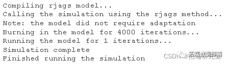
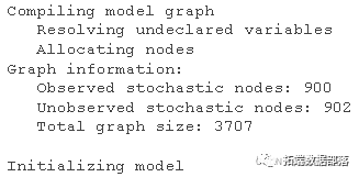
Ready to run JAGS!
# Calling JAGS from R
jags(nin = nb, woy = getwd() )
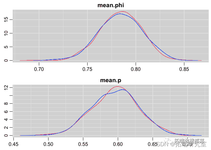
Summarize the posteriori and compare it with the values we used to simulate the data:
print(cj3)
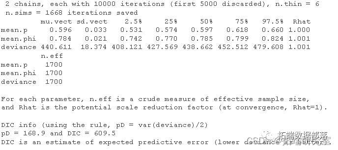
Very close!
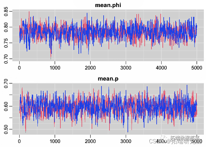
Tracking chart
trplot
Posterior distribution map
denplot