Lesson 11 convolutional neural network Advanced CNN
pytorch learning video - video link of station B: The final collection of PyTorch deep learning practice_ Beep beep beep_ bilibili
The following is the video content notes and source code. The notes are purely personal understanding. If there are errors, you are welcome to point them out.
1. GoogleNet
The network structure is shown in the figure,
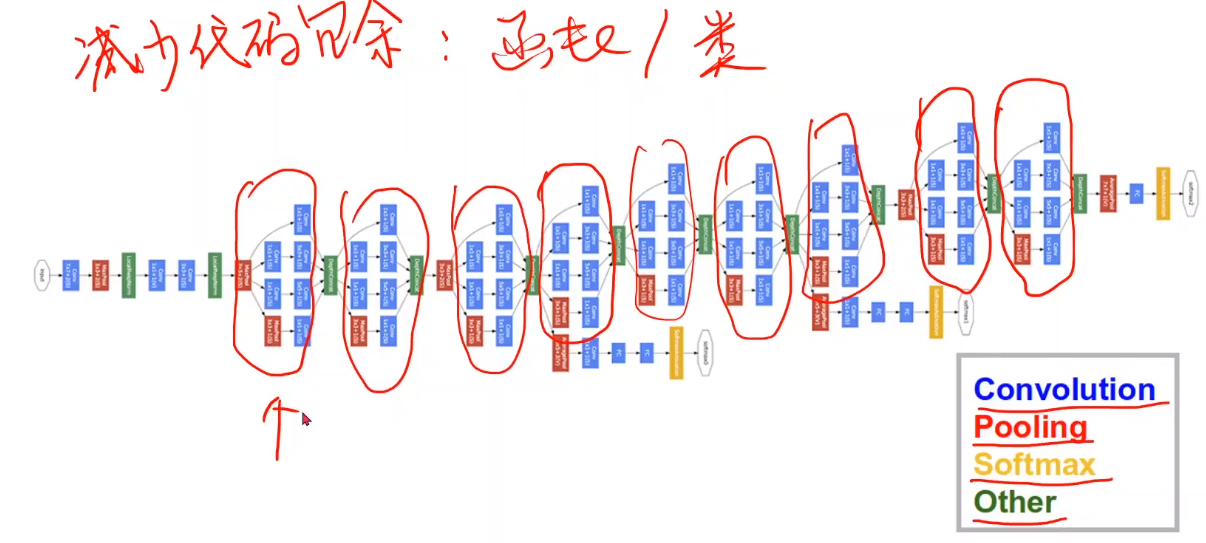
Google net is often used as the basic backbone network. The part circled in red in the figure is called the Inception block.
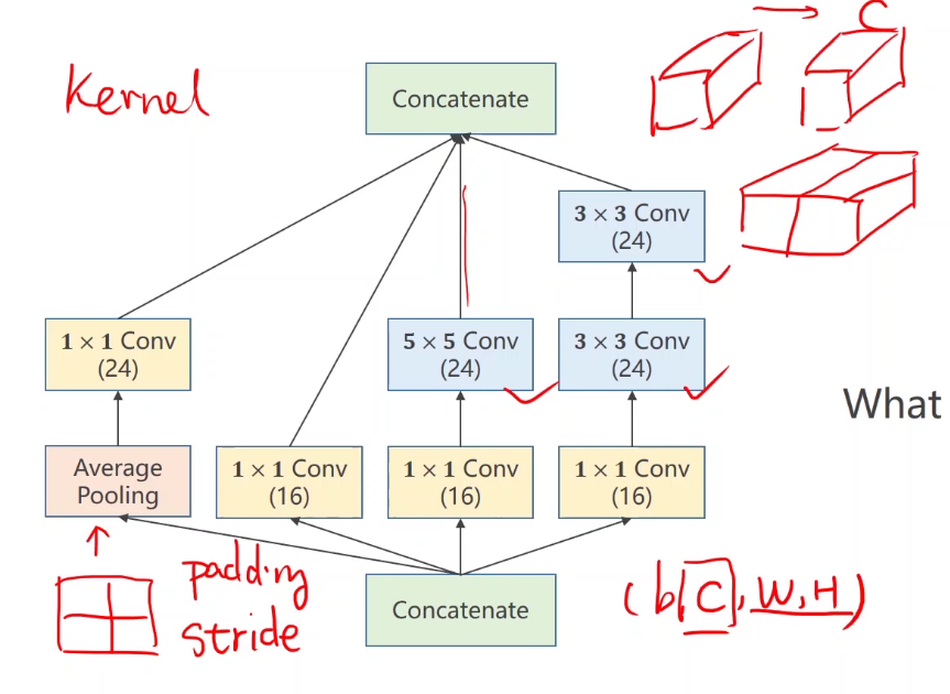
2. Perception module analysis
Do not know what kernel to select, use the convolution kernel once, give higher weight to the convolution kernel with better effect, and splice the results obtained by each convolution kernel.
-
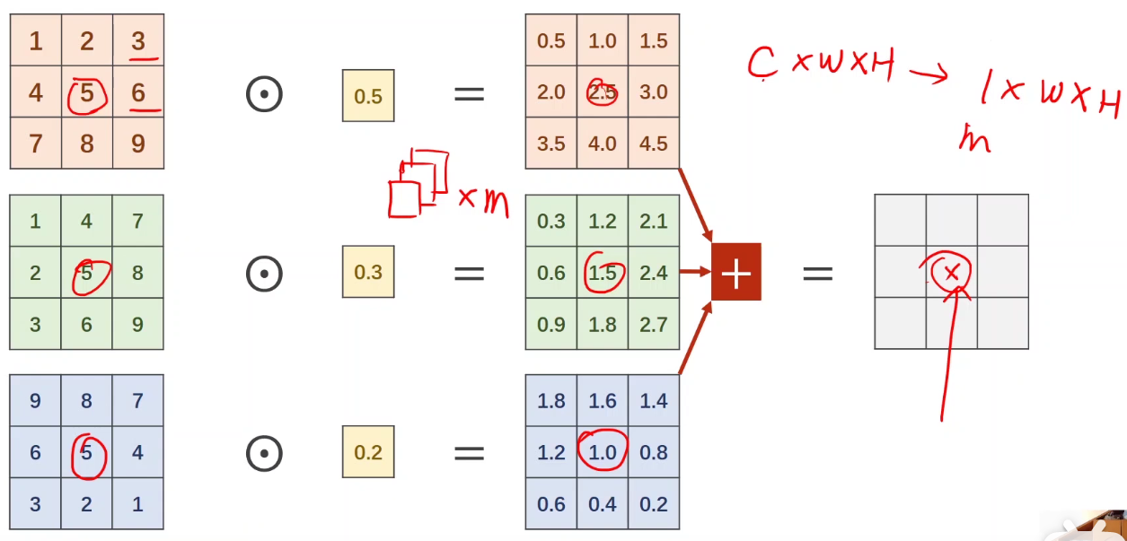
one × Convolution kernel analysis
It can be regarded as information fusion. One pixel value of the final feature map integrates the values of the first three channels.
The simplest example of information fusion - the examination compares the total score of each subject, which is not easy to compare in multiple dimensions.
Here is a channel transformation. The number of original channels is 3, and the number of new channels is the number of convolution kernels. The height and width remain unchanged.
-
effect
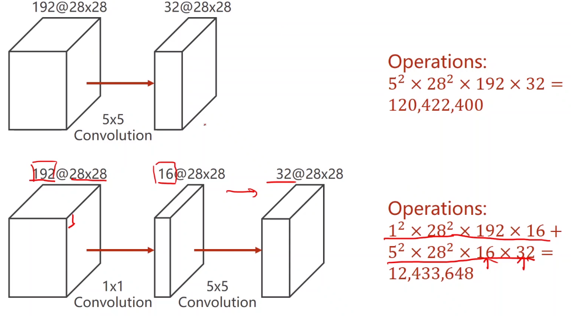
It can be used to reduce the amount of calculation, as shown in the figure:
If you convolute the original image directly, the amount of calculation is very large. If you use 1 first × The convolution kernel of 1 can reduce the number of channels, and then operate with the convolution kernel, which can reduce a lot of computation, as shown in the figure, plus 1 × After the convolution layer of 1, the amount of calculation is 1 / 10 of the original.
-
3. Implementation of inception module
As shown in the figure, there are four branches of the Inception block
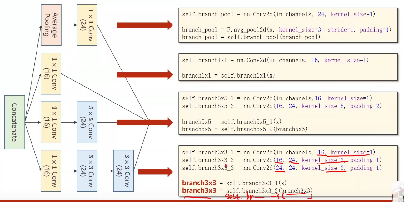
Implementation - advanced_cnn.py
import torch
from torch import nn
from torchvision import transforms
from torchvision import datasets
from torch.utils.data import DataLoader
import torch.nn.functional as F
import torch.optim as optim
import matplotlib.pyplot as plt
batch_size = 64
transform = transforms.Compose([
transforms.ToTensor(),
transforms.Normalize((0.1307, ), (0.3081, ))
])
train_dataset = datasets.MNIST(root='../dataset/mnist',
train=True,
download=True,
# The specified data is processed by transform
transform=transform)
train_loader = DataLoader(dataset=train_dataset,
batch_size=batch_size,
shuffle=True)
test_dataset = datasets.MNIST(root='../dataset/mnist',
train=False,
download=True,
transform=transform)
test_loader = DataLoader(dataset=test_dataset,
batch_size=batch_size,
shuffle=False)
# Define an Inception class, which will be used in the network
class InceptionA(nn.Module):
def __init__(self, in_channels):
super(InceptionA, self).__init__()
self.branch1X1 = nn.Conv2d(in_channels, 16, kernel_size=1)
# Set padding to ensure that the height and width of each branch output remain unchanged
self.branch5X5_1 = nn.Conv2d(in_channels, 16, kernel_size=1)
self.branch5X5_2 = nn.Conv2d(16, 24, kernel_size=5, padding=2)
self.branch3X3_1 = nn.Conv2d(in_channels, 16, kernel_size=1)
self.branch3X3_2 = nn.Conv2d(16, 24, kernel_size=3, padding=1)
self.branch3X3_3 = nn.Conv2d(24, 24, kernel_size=3, padding=1)
self.branch_pool = nn.Conv2d(in_channels, 24, kernel_size=1)
def forward(self, x):
branch1X1 = self.branch1X1(x)
branch5X5 = self.branch5X5_1(x)
branch5X5 = self.branch5X5_2(branch5X5)
branch3X3 = self.branch3X3_1(x)
branch3X3 = self.branch3X3_2(branch3X3)
branch3X3 = self.branch3X3_3(branch3X3)
branch_pool = F.avg_pool2d(x, kernel_size=3, stride=1, padding=1)
branch_pool = self.branch_pool(branch_pool)
outputs = [branch1X1, branch5X5, branch3X3, branch_pool]
# (b, c, w, h), dim=1 -- spliced with the first dimension channel
return torch.cat(outputs, dim=1)
# Define model
class Net(nn.Module):
def __init__(self):
super(Net, self).__init__()
self.conv1 = nn.Conv2d(1, 10, kernel_size=5)
self.conv2 = nn.Conv2d(88, 20, kernel_size=5)
self.incep1 = InceptionA(in_channels=10)
self.incep2 = InceptionA(in_channels=20)
self.mp = nn.MaxPool2d(2)
self.fc = nn.Linear(1408, 10)
def forward(self, x):
in_size = x.size(0)
x = F.relu(self.mp(self.conv1(x)))
x = self.incep1(x)
x = F.relu(self.mp(self.conv2(x)))
x = self.incep2(x)
x = x.view(in_size, -1)
x = self.fc(x)
return x
model = Net()
# Migrate the model to GPU and run it. cuda:0 means the 0th graphics card
device = torch.device("cuda:0" if torch.cuda.is_available() else "cpu")
print(torch.cuda.is_available())
model.to(device)
criterion = torch.nn.CrossEntropyLoss()
optimizer = optim.SGD(model.parameters(), lr=0.01, momentum=0.5)
# The training and testing processes are encapsulated in two functions respectively
def train(epoch):
running_loss = 0
for batch_idx, data in enumerate(train_loader, 0):
inputs, target = data
# The tensors to be calculated are also migrated to the GPU - input and output
inputs, target = inputs.to(device), target.to(device)
optimizer.zero_grad()
# Feedforward feedback update
outputs = model(inputs)
loss = criterion(outputs, target)
loss.backward()
optimizer.step()
running_loss += loss.item()
if batch_idx % 300 == 299:
print('[%d, %5d] loss: %.3f' % (epoch + 1, batch_idx + 1, running_loss / 300))
running_loss = 0
accuracy = []
def test():
correct = 0
total = 0
with torch.no_grad():
for data in test_loader:
images, labels = data
# The tensor in the test is also migrated to the GPU
images, labels = images.to(device), labels.to(device)
outputs = model(images)
_, predicted = torch.max(outputs.data, dim=1)
total += labels.size(0)
correct += (predicted == labels).sum().item()
print('Accuracy on test set: %d %%' % (100 * correct / total))
accuracy.append(100 * correct / total)
if __name__ == '__main__':
for epoch in range(10):
train(epoch)
test()
print(accuracy)
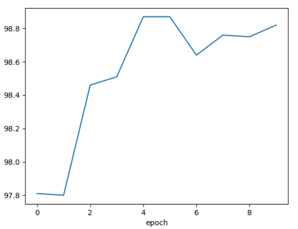
plt.plot(range(10), accuracy)
plt.xlabel("epoch")
plt.ylabel("Accuracy")
plt.show()
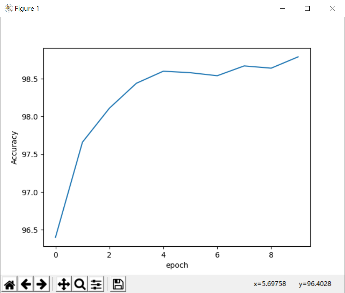
result:
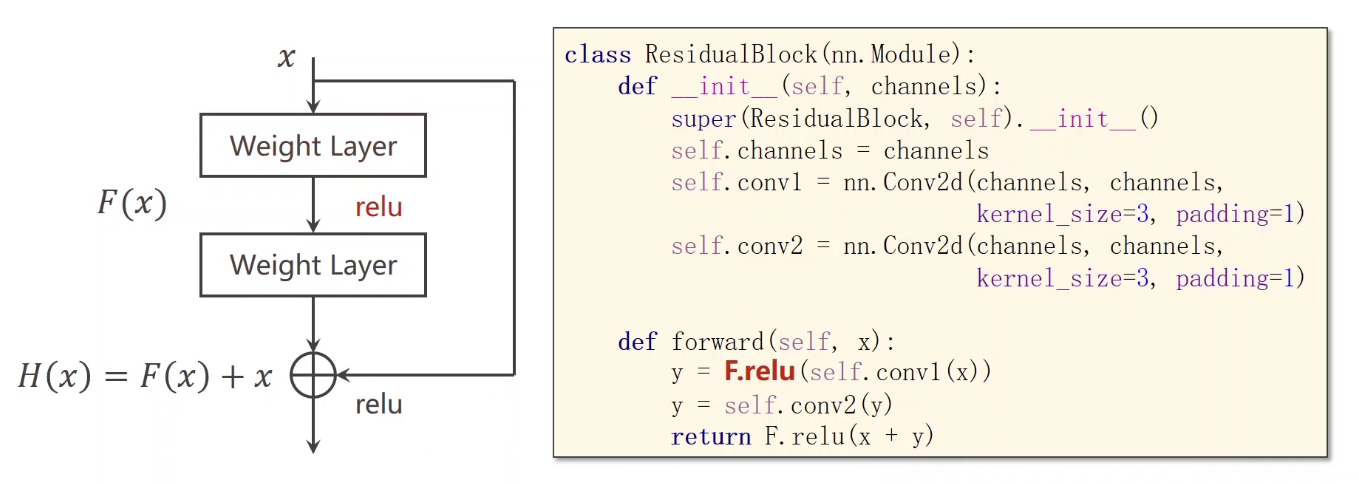
4. Residual network
The difference between ordinary network and residual network. Before convolution activation, the residual network activates the input and output of this layer as the whole output.
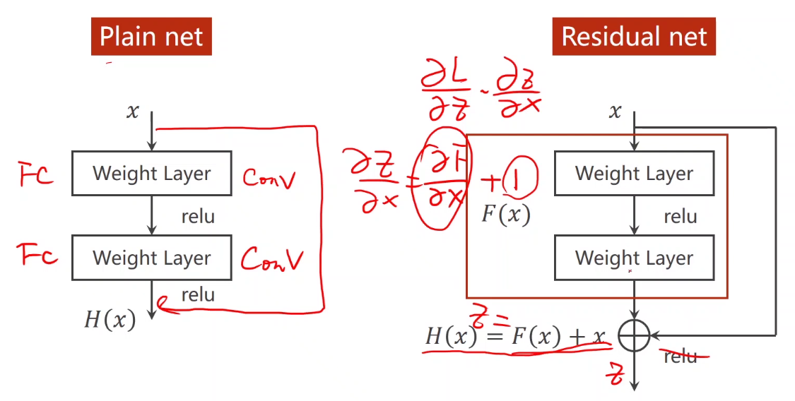
definition:
Implementation - residual py
import torch
from torch import nn
from torchvision import transforms
from torchvision import datasets
from torch.utils.data import DataLoader
import torch.nn.functional as F
import torch.optim as optim
import matplotlib.pyplot as plt

batch_size = 64
transform = transforms.Compose([
    transforms.ToTensor(),
    transforms.Normalize((0.1307, ), (0.3081, ))
])

train_dataset = datasets.MNIST(root='../dataset/mnist',
                               train=True,
                               download=True,
                               # The specified data is processed by transform
                               transform=transform)
train_loader = DataLoader(dataset=train_dataset,
                          batch_size=batch_size,
                          shuffle=True)

test_dataset = datasets.MNIST(root='../dataset/mnist',
                              train=False,
                              download=True,
                              transform=transform)
test_loader = DataLoader(dataset=test_dataset,
                         batch_size=batch_size,
                         shuffle=False)


# Define a residual module class
class ResidualBlock(nn.Module):
    def __init__(self, channels):
        super(ResidualBlock, self).__init__()
        self.channels = channels
        self.conv1 = nn.Conv2d(channels, channels, kernel_size=3, padding=1)
        self.conv2 = nn.Conv2d(channels, channels, kernel_size=3, padding=1)

    def forward(self, x):
        y = F.relu(self.conv1(x))
        y = self.conv2(y)
        return F.relu(x + y)


# Define model
class Net(nn.Module):
    def __init__(self):
        super(Net, self).__init__()
        self.conv1 = nn.Conv2d(1,16, kernel_size=5)
        self.conv2 = nn.Conv2d(16, 32, kernel_size=5)
        self.mp = nn.MaxPool2d(2)

        self.rblock1 = ResidualBlock(16)
        self.rblock2 = ResidualBlock(32)

        self.fc = nn.Linear(512, 10)

    def forward(self, x):
        in_size = x.size(0)
        x = self.mp(F.relu(self.conv1(x)))
        x = self.rblock1(x)
        x = self.mp(F.relu(self.conv2(x)))
        x = self.rblock2(x)
        x = x.view(in_size, -1)
        x = self.fc(x)
        return x


model = Net()
# Migrate the model to GPU and run it. cuda:0 means the 0th graphics card
device = torch.device("cuda:0" if torch.cuda.is_available() else "cpu")
print(torch.cuda.is_available())
model.to(device)

criterion = torch.nn.CrossEntropyLoss()
optimizer = optim.SGD(model.parameters(), lr=0.01, momentum=0.5)


# The training and testing processes are encapsulated in two functions respectively
def train(epoch):
    running_loss = 0
    for batch_idx, data in enumerate(train_loader, 0):
        inputs, target = data
        # The tensors to be calculated are also migrated to the GPU - input and output
        inputs, target = inputs.to(device), target.to(device)
        optimizer.zero_grad()

        # Feedforward feedback update
        outputs = model(inputs)
        loss = criterion(outputs, target)
        loss.backward()
        optimizer.step()

        running_loss += loss.item()
        if batch_idx % 300 == 299:
            print('[%d, %5d] loss: %.3f' % (epoch + 1, batch_idx + 1, running_loss / 300))
            running_loss = 0

accuracy = []
def test():
    correct = 0
    total = 0
    with torch.no_grad():
        for data in test_loader:
            images, labels = data
            # The tensor in the test is also migrated to the GPU
            images, labels = images.to(device), labels.to(device)
            outputs = model(images)
            _, predicted = torch.max(outputs.data, dim=1)
            total += labels.size(0)
            # ?? How to compare equality
            # print(predicted)
            # print(labels)
            # print('predicted == labels', predicted == labels)
            # Comparing the two tensors, we can get the number of equal elements (i.e. the number of correctly predicted elements in a batch)
            correct += (predicted == labels).sum().item()
            # print('correct______', correct)
    print('Accuracy on test  set: %d %%' % (100 * correct / total))
    accuracy.append(100 * correct / total)


if __name__ == '__main__':
    for epoch in range(10):
        train(epoch)
        test()
    print(accuracy)
    plt.plot(range(10), accuracy)
    plt.xlabel("epoch")
    plt.ylabel("Accuracy")
    plt.show()
result: