preface

At the end of the last article, we also reserved a few questions. Firstly, we will use the modified laida criterion to screen outliers based on the actual data; In addition, for the processing of outliers, when the data does not clearly obey what distribution (or even approximate normal distribution, but generally approximate normal distribution in case of a large amount of data), the effect of screening outliers by using the principle of probability distribution will be slightly worse. Instead, systematic methods are used to screen outliers.

1: The effectiveness of the modified laida criterion is verified in multiple directions based on the actual data

• Firstly, the feature results based on normal data extraction mentioned in the second article are reviewed
  Generalization of convenient and effective feature extraction method in multi classification

  Index(['alcohol', 'total sulfur dioxide','volatile acidity', 'fixed acidity',
       'citric acid', 'residual sugar','sulphates', 'free sulfur dioxide',
        'pH', 'density', 'chlorides'],dtype='object') 

• Insert outlier data into dataset

Based on this data, we artificially add 30 outliers on the random position of each dimension data in 1500 samples through the code. The value of outliers is 5-25 times of the original value, and let the random number obey uniform distribution.

import random as rd
ret_all = []
for i in range(data.shape[1] - 1):##Traverse each column
    ret = []
    for j in range(30):##30 cycles
        r = rd.randint(1, data.shape[0])
        mul = rd.uniform(5, 25)#Take a number between 5 and 25 at random
        data.iloc[r,i] = data.iloc[r,i] * mul
        ret.append(r)
    ret_all.append(ret)

Then we run programs separately. The first program is the screening result without any processing when the outlier exists; The second program is the screening result of the data set after ordinary laida (de extremum), and the third program is the screening result of the data set processed by the modified laida( Revise the laida code. Please see the previous article).

When outliers exist
    Absolute distance after standardization 
      0   1.214867  1   1.216809  2   1.263637  
      3   1.183755  4   1.232970  5   1.086079  
      6   1.126362  7   1.381525  8   1.377077  
      9   1.259793  10  1.350094  
Index(['density', 'pH', 'alcohol', 'citric acid', 'sulphates', 'chlorides',
       'volatile acidity', 'fixed acidity', 'residual sugar',
       'total sulfur dioxide', 'free sulfur dioxide'],dtype='object')

Results of abnormal points screened by ordinary laida (de extremum)
    Absolute distance after standardization  
     0   1.178103  1   0.709496  2   1.635919  
     3   1.050437  4   0.936631  5   1.042880  
     6   1.193319  7   1.406353  8   1.350272  
     9   1.122081  10  1.490989  
Index(['citric acid', 'alcohol', 'density', 'pH', 'total sulfur dioxide',
       'fixed acidity', 'sulphates', 'residual sugar', 'free sulfur dioxide',
       'chlorides', 'volatile acidity'],dtype='object')

Results after screening through the modified version of laida
    Absolute distance after standardization  
      0   1.494828  1   1.338518  2   1.322476  
      3   1.266294  4   1.229666  5   1.344060  
      6   1.391119  7   1.140193  8   1.279546  
      9   1.310606  10  1.380547  
Index(['fixed acidity','total sulfur dioxide','alcohol', 'free sulfur dioxide',
       'volatile acidity','citric acid', 'sulphates', 'pH',
       'residual sugar' 'chlorides', 'density'],dtype='object')

• Visual analysis

As like as two peas, we can see that the revised version of the rule is used to handle the data set containing abnormal points, and then the distance feature is selected to calculate the result. The result is very similar to the original dataset without exception points. The top and the top ranking names are almost the same. However, there are obvious disadvantages in the extracted features of the unprocessed exception data sets and those processed by the general criteria (de extremum), and many features that should be ranked at the back are ranked at the top.

• Validity judgment
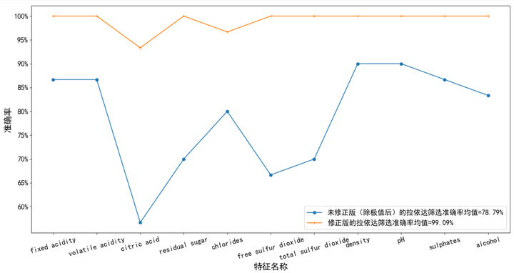
  We define the accuracy of filtering r t = n sieve choose Out of n real Occasion Save stay of × 100 % r_{t}=\frac{n {filtered} {n {actual}} \ times 100 \% rt = n actual, n filtered × 100%, here n real Occasion Save stay of = 30 n_ {actual} = 30 n actual = 30. Figure 1 below shows the accuracy of filtering outliers by the two methods under each dimension. Obviously, it can be seen that the modified laida criterion is better than the ordinary laida criterion (de extremum).
  

Figure 1

• Summary

So far, the comprehensive modeling analysis of outlier model based on probability distribution + distance screening feature model can be said to be over for a while. From the previous experiments, it can be seen that all the experimental results are within the scope of our theoretical analysis, which directly proves that the relevant model we proposed before is effective and convenient!

2: Outlier screening method based on Data Center

• explain

Here, all dimension data of a sample are regarded as one object (feature extraction and dimensionality reduction can be carried out first for high latitude). The final screening result is directly the index value of the sample, rather than which dimension data corresponding to a sample is abnormal. This method often involves a lot of computation, but has strong applicability.

• Implementation steps

1. Set sample data size A m , n = m × n A_{m,n}=m\times n Am,n​=m×n ( m m m samples, n n n-dimensional feature length) to prevent the deviation caused by the magnitude of dimensional data, we first standardize or normalize the data. The normalization processing includes: B m , n = ( A m , n − m i n ( A ) ) / ( m a x ( A ) − m i n ( A ) ) B_{m,n}=(A_{m,n}-min(A))/(max(A)-min(A)) Bm,n​=(Am,n​−min(A))/(max(A)−min(A)) ,
2. Solving matrix B m , n B_{m,n} Bm,n = the center point of each dimension is C = ( C 1 , C 2 , . . . C n ) C=(C_{1},C_{2},...C_{n}) C=(C1, C2,... Cn), let the matrix B B B each row of data is different from the corresponding center point value, i.e H i 1 ≤ i ≤ m , j = B i 1 ≤ i ≤ m , j − C j H_{i_{1\leq i\leq m},j}=B_{i_{1\leq i\leq m},j}-C_{j} Hi1≤i≤m​,j​=Bi1≤i≤m​,j​−Cj​ ,
3. Re pairing matrix H H H do each line p p p-order norm operation, i.e H i = ( ∑ j m ∣ H i , j ∣ p ) 1 p H_{i}=\left( \sum_{j}^{m}{|H_{i,j}|^{p}} \right)^{\frac{1}{p}} Hi​=(∑jm​∣Hi,j​∣p)p1​ . The premise is that each line p p The moment of order p is bounded, i.e E ∣ H i , j ∣ p < ∞ E{|H_{i,j}|^{p}} <\infty E∣Hi,j​∣p<∞ ，
4. Re pair vector H i H_{i} The attribute value of Hi ， can be selected for constraint processing H i ˉ = H i m e a n / m a x / m e d i a n ( H i ) \bar{H_{i}}=\frac{H_{i}}{mean/max/median(H_{i})} Hi​ˉ​=mean/max/median(Hi​)Hi​​ ,
5. Finally, we select the threshold α \alpha α ， vector H i H_{i} Element in Hi is greater than α \alpha α Will be eliminated.

• Here, the value of center vector C is a difficult point. How to choose it?

First, the data set is directly averaged. Generally, the data will be standardized to prevent the difference caused by the order of magnitude. Then we can go further, that is, then take the mean,
Second, we can find the cluster center by clustering. We can use semi supervised clustering, unsupervised clustering and so on.

3: Finding data centers based on quantiles

Let's start with a simple method, select the quantile of the data set, and then take the mean value of each dimension.

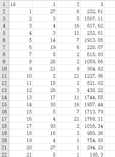
• Find out the 10% quantile value and 95% quantile value of each dimension data. We only take all the data between the two. The data source (excerpt) is shown in Figure 2 below:

Figure 2

Then through the following code, we get the center of each dimension of the data.

mean_ls = []
for i in data_temp.columns:
    loc_down = np.percentile(data_temp[i],10)
    loc_up = np.percentile(data_temp[i],95)
    data_t = data_temp[i][(data_temp[i] > loc_down) & (data_temp[i] <= loc_up)]#The data is judged and filtered
    mean_ls.append(data_t.mean())

Then, the steps in Section 2 are realized one by one:

data_temp = (data - data.min()) / (data.max() - data.min())
def pick_discrete_points(threshold,p=2):##The relative distance threshold is set to 2
    df_ls = []
    for i in data_temp.columns:
        loc_down = np.percentile(data_temp[i],10)
        loc_up = np.percentile(data_temp[i],95)
        data_t = data_temp[i][(data_temp[i] > loc_down) & (data_temp[i] <= loc_up)]
        norm_tmp = data_temp[i] - data_t.mean()#Subtract the data center value from each row
        df_ls.append(norm_tmp)
    df_f = pd.concat(df_ls,axis=1)
    norm_new = df_f.apply(np.linalg.norm,ord=p,axis=1)##Calculate the p-order norm of each row
    norm_fin = norm_new / norm_new.mean()##Data range constraints

    norm_fin[norm_fin <= threshold].plot(style='bo',label='Normal point')##Normal point
    discrete_points = norm_fin[norm_fin > threshold]
    discrete_points.plot(style='ro',figsize=(15,8),label='Outlier')##Discrete point

    y = [threshold for i in range(len(norm_fin))]##Standard line
    print(len(discrete_points.index),discrete_points.index)
    plt.plot(y,'orange',label='Relative standard line')
    plt.xlabel('number',fontsize=18)
    plt.ylabel('Relative distance',fontsize=18)
    plt.tick_params(labelsize=18)
    plt.annotate('Outlier(%s,%.3f)'%(discrete_points.index[5],norm_fin.loc[discrete_points.index[5]]), xy=(discrete_points.index[5],norm_fin.loc[discrete_points.index[5]]),
                 xytext=(300,3), arrowprops=dict(arrowstyle="fancy"),fontsize=20)
    plt.legend(fontsize=15)
    plt.show()
pick_discrete_points(2)

Figure 3

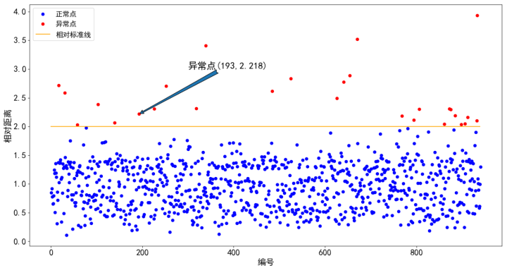
From Figure 3, we can clearly observe the overall distribution of nearly 1000 sample data according to the relative distance value. Our outlier data is above the standard line. There are many options for how to deal with the found outlier data. We mentioned it in the previous article and will not repeat it here.

4: Summary and Prospect

• In this article, we mainly explained the effectiveness of the modified laida criterion for outlier screening based on the actual data, and also did an outlier screening by using the systematic method, and finally visualized the screening results. From the above results, our method and model are still more effective.
• For the outlier screening of systematic methods, we mentioned that the origin of data center can be based on semi supervised clustering and unsupervised clustering. How can I realize these processes and prove to be effective methods? This is also a good discussion content. We will give the discussion conclusions in the subsequent articles.
• In the next article, we will temporarily put on the content of machine learning and data mining. We will talk about the common discrete simulation of random processes. The theory of random processes is very profound. We will briefly touch on a little, mainly numerical simulation, including discrete Markov chain, Poisson process and so on.