Realization of 3.2 Linear Regression from Zero
Now that you know the background of linear regression, we can begin to implement it. Although a strong framework for in-depth learning can reduce a lot of repetitive work, relying too much on its convenience will make it difficult to understand how in-depth learning works. Therefore, this section describes how to train a linear regression using only Tensor and Gradient Tape.
First, import the packages or modules needed for the experiments in this section, where the matplotlib package can be used for mapping and set up for embedded display.
%matplotlib inline
import tensorflow as tf
print(tf.__version__)
from matplotlib import pyplot as plt
import random
output
2.0.0
3.2. 1 Generate dataset
We construct a simple manual training dataset that allows us to visually compare the differences between the learned parameters and the real model parameters. Set the number of training dataset samples to 1000 and the number of inputs (the number of features) to 2. Given the randomly generated batch sample characteristics X ∈ R 1000 × 2 \boldsymbol{X} \in \mathbb{R}^{1000 \times 2} X < R1000 × 2, we use the real weight of the linear regression model w = [ 2 , − 3.4 ] ⊤ \boldsymbol{w} = [2, -3.4]^\top w=[2,3.4], and deviation b = 4.2 b = 4.2 b=4.2, and a random noise term ϵ \epsilon ϵ To generate labels y = X w + b + ϵ \boldsymbol{y} = \boldsymbol{X}\boldsymbol{w} + b + \epsilon y=Xw+b+ϵ
Where the noise item ϵ \epsilon ϵ It obeys a normal distribution with a mean of 0 and a standard deviation of 0.01. Noise represents meaningless interference in the dataset. Next, let's generate the dataset.
num_inputs = 2
num_examples = 1000
true_w = [2, -3.4]
true_b = 4.2
features = tf.random.normal((num_examples, num_inputs),stddev = 1)
labels = true_w[0] * features[:,0] + true_w[1] * features[:,1] + true_b
labels += tf.random.normal(labels.shape,stddev=0.01)
Note that each row of features is a vector of length 2, while each row of labels is a vector of length 1 (scalar).
print(features[0])
print(labels[0])
Output:
tf.Tensor([1.1232399  0.14090918], shape=(2,), dtype=float32)
tf.Tensor(5.9658055, shape=(), dtype=float32)
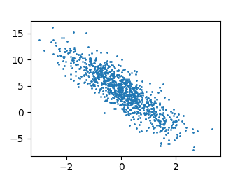
By generating a scatterplot of the second feature features[:, 1] and labels labels, the linear relationship between them can be more visually observed.
def set_figsize(figsize=(3.5, 2.5)):
    plt.rcParams['figure.figsize'] = figsize

set_figsize()
plt.scatter(features[:, 1], labels, 1)
3.2. 2 Read data
When training a model, we need to traverse the dataset and constantly read small batches of data samples. Here we define a function that returns batch_each time The characteristics and labels of size (batch size) random samples.
def data_iter(batch_size, features, labels):
    num_examples = len(features)
    indices = list(range(num_examples))
    random.shuffle(indices)
    for i in range(0, num_examples, batch_size):
        j = indices[i: min(i+batch_size, num_examples)]
        yield tf.gather(features, axis=0, indices=j), tf.gather(labels, axis=0, indices=j)
Let's read the first small batch data sample and print it. The characteristic shape of each batch is (10, 2), corresponding to the batch size and the number of inputs; Label shape is batch size.
batch_size = 10

for X, y in data_iter(batch_size, features, labels):
    print(X, y)
    break
 Output:

tf.Tensor(
[[ 0.04718596 -1.5959413 ]
 [ 0.3889716  -1.5288432 ]
 [-1.8489572   1.66422   ]
 [-1.3978077  -0.85818154]
 [-0.36940867 -0.619267  ]
 [-0.15660426  1.1231796 ]
 [ 0.89411694  1.5499148 ]
 [ 1.9971682  -0.56981105]
 [-2.1852891   0.18805206]
 [ 1.3222371  -1.0301086 ]], shape=(10, 2), dtype=float32) tf.Tensor(
[ 9.738684   10.164594   -5.15065     4.3305573   5.568048    0.06494669
  0.7251317  10.128626   -0.8036391  10.343082  ], shape=(10,), dtype=float32)
3.2. 3 Initialize model parameters
We initialize the weight to a normal random number with a mean of 0 and a standard deviation of 0.01, and the deviation to 0.
w = tf.Variable(tf.random.normal((num_inputs, 1), stddev=0.01))
b = tf.Variable(tf.zeros((1,)))
3.2. 4 Define the model
Below is the implementation of a vector calculation expression for linear regression. We use the matmul function for matrix multiplication.
def linreg(X, w, b):
    return tf.matmul(X, w) + b
3.2. 5 Define loss function
We use the square loss described in the previous section to define the loss function for linear regression. In implementation, we need to transform the true value y into the predicted value y_ The shape of the hat. The following function also returns the same result as y_ The hats have the same shape.
def squared_loss(y_hat, y):
    return (y_hat - tf.reshape(y, y_hat.shape)) ** 2 /2
3.2. 6 Definition optimization algorithm
The sgd function below implements the small-batch random gradient descent algorithm described in the previous section. It optimizes the loss function by iterating over the model parameters. Here the gradient calculated by the automatic gradient module is the sum of the gradients of a batch of samples. We divide it by the batch size to get the average.
def sgd(params, lr, batch_size, grads):
    """Mini-batch stochastic gradient descent."""
    for i, param in enumerate(params):
        param.assign_sub(lr * grads[i] / batch_size)
3.2. 7 Training Model
In the training, we will iterate over the model parameters several times. In each iteration, we calculate a small batch random gradient by invoking the inverse function t.gradients based on the small batch data samples (Feature X and Label y) currently read, and invoke the optimization algorithm sgd iteration model parameters. Since we previously set the batch size to 10, the shape of each small batch loss l is (10, 1). Recall the section on finding gradients automatically. Since variable l is not a scalar, we can call reduce_sum() sums it up to a scalar and runs t.gradients to get the gradient of the variable with respect to the model parameters. Be careful not to forget to zero out the gradient of the parameter after each parameter update.
In an iterative cycle (epoch), we will iterate through the data_iter function completely and use it once for all samples in the training dataset (Assuming that the number of samples can be divided by the batch size). Here, the number of iteration cycles num_epochs and the learning rate lr are hyperparameters, set to 3 and 0.03, respectively. In practice, most of the hyperparameters need to be continuously adjusted through trial and error. Although a model with a larger number of iteration cycles may be more effective, the training time may be too long. As for the impact of learning rate on the model, I They are described in more detail in the following chapter, Optimizing Algorithms.
lr = 0.03
num_epochs = 3
net = linreg
loss = squared_loss

for epoch in range(num_epochs):
    for X, y in data_iter(batch_size, features, labels):
        with tf.GradientTape() as t:
            t.watch([w,b])
            l = tf.reduce_sum(loss(net(X, w, b), y))
        grads = t.gradient(l, [w, b])
        sgd([w, b], lr, batch_size, grads)
    train_l = loss(net(features, w, b), labels)
    print('epoch %d, loss %f' % (epoch + 1, tf.reduce_mean(train_l)))
Output:
epoch 1, loss 0.028907 epoch 2, loss 0.000101 epoch 3, loss 0.000049
After the training is completed, we can compare the parameters we learned with the actual parameters used to generate the training set. They should be close together.
print(true_w, w)
print(true_b, b)
Output:
([2, -3.4], <tf.Variable 'Variable:0' shape=(2, 1) dtype=float32, numpy= array([[ 1.9994558], [-3.3993363]],dtype=float32)>)
(4.2, <tf.Variable 'Variable:0' shape=(1,) dtype=float32, numpy=array([4.199041], dtype=float32)>)