Original link: http://tecdat.cn/?p=24761
This document uses some exploratory data analysis to develop the rating curve and flow prediction of the river. The purpose is to create and update rating curves using (1) instantaneous flow measured during periodic deployment of bottom mounted units and (2) instantaneous depth measurements from water level data recorders deployed in rivers for a long time. The rating curve will be used to calculate the flow during the deployment of HOBO pressure sensor (about 1 year). The resulting data will be used to create and verify the regression and DAR flow estimation of the river over a period of 10-15 years.
introduce
Rating curve
Due to the high cost associated with continuous measurement of river flow, it is best to use river height measurement to estimate flow. The water flow height can be measured continuously by using the pressure sensor. When supplemented by periodic flow measurement, the power function can correlate river height and flow (Venetis):
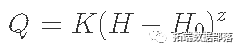
Where: Q represents steady-state emission, H represents flow height (stage), H0 is zero emission stage; K and z are rating curve constants. According to convention, Q and H usually undergo logarithmic transformation before parameter estimation.
When the rising and falling stages of the river water level hydrograph lead to different flows at the same river height, unstable flow will occur. The resulting rating curve affected by lag will appear as a cycle rather than a line. The modified Jones formula described by Petersen - Ø verleir and Zakwan may have been used:
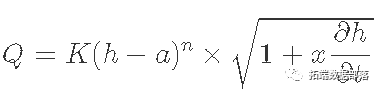
Where Q is the flow and h is the river height. Partial first derivative

Using the finite difference approximation J:
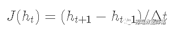
Where ht is the flow height at time t, Δ T is the time interval. This can be considered as the slope or instantaneous rate of change of the function between river height and time, which is estimated using the measured river height value. K. a, n and x are rating curve constants.
Many different methods can be used to solve the rated curve parameters. We use nonlinear least squares regression to minimize the sum of squares of residuals (SSE) of rating curve parameters. The residual SSE is calculated as follows:
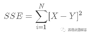
Where X is the measured value and Y is the predicted value. The nonlinear optimization method searches for parameter combinations to minimize the objective function (in this case, it is residual SSE). Peterson uses Nelder Mead algorithm to solve Jones formula. Zaguan uses generalized gradient reduction and genetic algorithm to propose nonlinear optimization methods. Most methods need to carefully plan the initial value of parameters that are a little close to the global minimum, or there is a risk of identifying alternative local minimum values. In order to reduce the possibility of convergence of local minimum values , R provides the function of iterating nonlinear least squares optimization on many different starting values (Padfield and Matheson)
Uncontrolled flow estimation
The rating curve allows the development of daily flow records during the time period when the flow depth data logger is deployed. However, when the site is not enabled, the estimation of daily traffic requires additional information. Statistical information transfer and empirical regression are two relatively simple methods that can be used to estimate the flow in improperly measured watersheds. The statistical transfer program uses the hypothetical relationship between area and runoff to simply transfer the flow duration curve or daily flow value from the measured watershed to the unmeasured watershed. The most commonly used statistical transfer method is watershed area ratio. Using the watershed area ratio, the daily flow is transferred from one watershed to another by multiplying the area ratio by the daily flow:
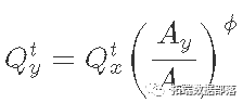
Among them,

Is the flow that predicts basin y and time t,

Is to measure the flow at basin x and time tt, and

Is the area ratio of the basin. Parameters ϕ Usually equal to 1 (Asquith, Roussel, and Vrabel). However, asquis, Russell, and frabel provide information for watershed area ratios when applied in Texas ϕ Empirical estimates. With available short-term flow records, the drainage area ratio method can be used to evaluate the performance of various flow instruments. In addition, it can be developed using nonlinear least squares method ϕ Local value of. If the main output is the flow duration curve, the main concern is that the candidate quantities have similar runoff dependent variables and are within a reasonable distance from the untreated watershed. However, if the main output includes daily traffic estimation, it is more important to have candidate gauges with the same traffic exceedance probability time.
The method based on empirical regression requires a period of measured flow and some predictive variables to estimate the runoff dependent variables. Generally, the daily rainfall data is used to fit the regression model to the measured flow data:
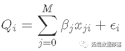
Where Qi is the predicted emission on day i, β Is the coefficient of the j-th variable, and x is the predicted variable value on day i. Hypothetical error term ϵ i is normally distributed near the mean zero. Using simple linear or multiple linear regression Q, logarithmic transformation is usually performed before estimating regression coefficients. If the relationship between the prediction variable and the dependent variable is expected to be a nonlinear polynomial, a term may be included. However, the extension of linear regression called generalized additive model allows these nonlinear terms to be fitted to the data relatively easily. For the generalized additive model, the dependent variable depends on the sum of the smoothing functions applied to each predictive variable. In addition, the generalized additive model can fit the dependent variables of error distribution with non normal distribution. However, compared with the first mock exam, the generalized additive model is more difficult to explain because of the lack of a single model coefficient. Therefore, the influence of each individual smoothing function on the mean value of the dependent variable is usually conveyed graphically.
method
data acquisition
The data comes from the water level data recorder. An additional datalogger was deployed to provide ambient atmospheric pressure correction for the datalogger deployed underwater. From 2020-03-02 to 2021 -.. -, The water level data logger is deployed almost continuously and is set to record the water level every 15 minutes.
## Make a list of files to import

                     list.files(path = here("Data

##Create a blank tibble to fill in
 tibble()


## Traverse the file path to read each file
for (i in fihs) {
  x <- read_csv(

    copes
  bind_rows(hf, x)
  rm(x)
Table 1: summary statistics of 15 minute flow levels measured at each site

ggplot(hdf) +
  geom_line+
  facet_wrap +
  scale\_x\_datetim+
  scale_y +
  guid +
  th +
  theme
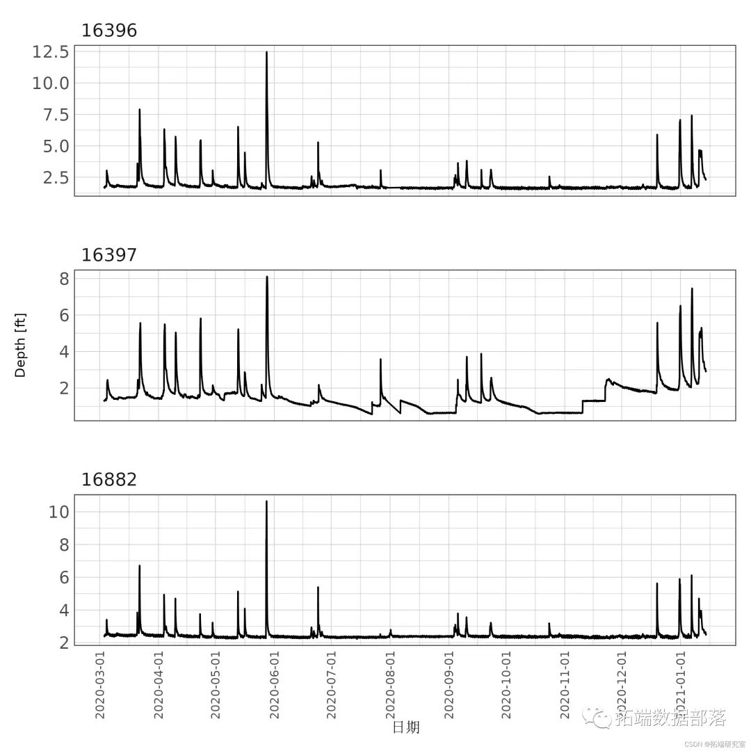
Figure 1: 15 minute interval flow depth record for each station.
Periodic flow measurements are made at each SWQM station using a bottom mounted flowmeter. Measure the cross-sectional area, water flow height and velocity. Using these measurements, the device uses the exponential velocity method to report instantaneous flow. The flow measurement equipment is deployed for several days at a time to capture the complete hydrological hydrograph under different flow conditions of each station. Only two flowmeters are available, so they are deployed alternately between sites. In addition, one equipment stopped working and was repaired for several months. Record the flow at 15 minute intervals.
In the process of data exploration, there is obviously too much noise in the low traffic data of each station. During stagnation or near stagnation conditions, the Doppler flowmeter records highly variable flow rates and reports unrealistic flows. Very low or stagnant flow periods are removed from the data record due to excessive data noise. Future deployment will need to consider under what conditions long-term deployment is appropriate. For small streams like this, regular storm stream deployment may be the most appropriate deployment.
## Make a list of files to import
file_paths <- paste0(he ".csv"))

##Create a blank tibble to fill in
iq <- tibble()

## Traverse the file path to read each file
for (i in file_paths) {
  x <- read_csv
  file <- i
  idf <- bind_rows
  rm
}


iqdf <- iqdf %>%
  ## Use \ ` dplyr:: \ ` to specify the rename function to use, just in case
  dplyr::rename(Sam)


ggplot(iqdf)+
  geom_point(aes(Dme, Flow), alpha = 0.2) +
  facet_wrap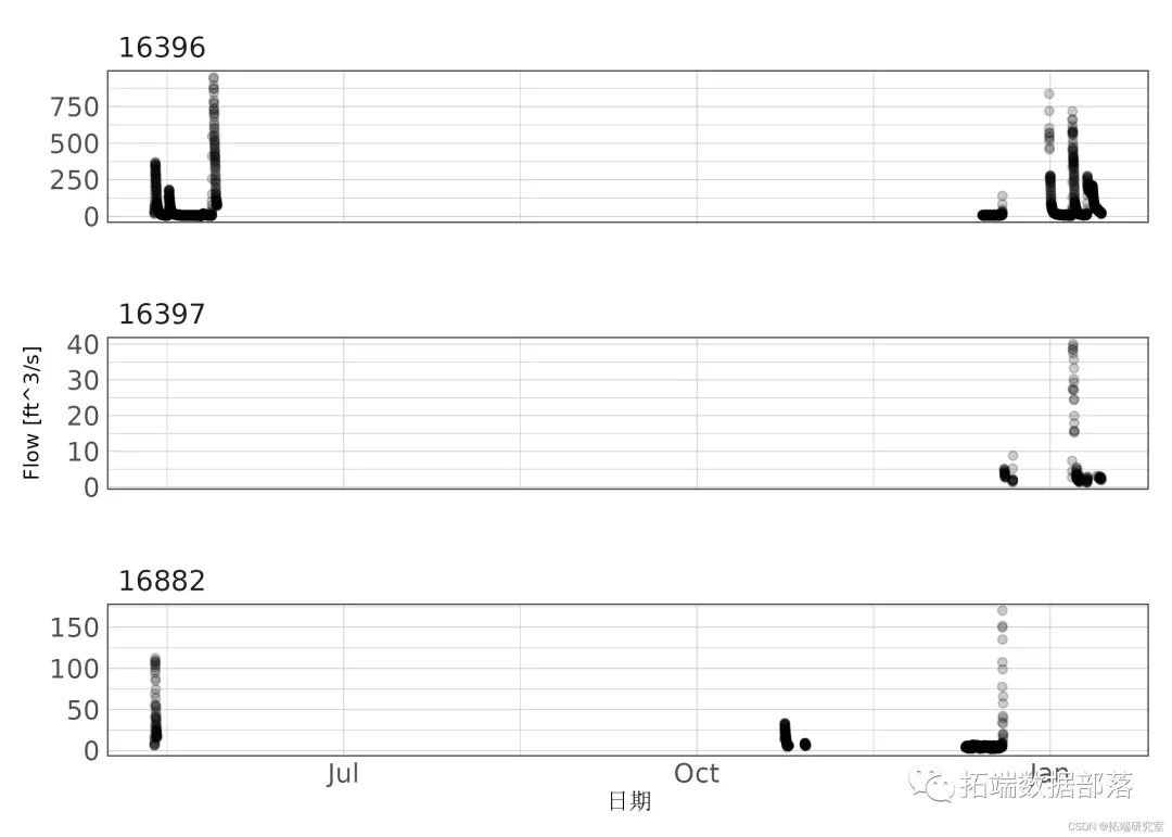
Figure 2: cycle of recording data at each site.
## In order to combine the measurement depth with the flow rate measurement of IQ
## We need to interpolate the measured depth to every minute because the depth is offset. Then we can connect the data. We will use linear interpolation.


##Run interpolation on each site using purrr::map
hdf %>%
  split%>%
  map %>%
  bind_row %>%
  as_tibble
##This is the data framework we want to develop the rating curve.
idf %>%
  left_join %>%
  select %>%
  mutate -> iqdf
Rating curve development
Due to plant growth, plant death, deposition, erosion and other processes, the conditions of Hanoi and river banks will change throughout the year. These changing conditions may require the development of multiple rating curves. Exploratory data analysis is used to determine the possibility of changing periods and lags affecting the rating curve. Once the rating curve period and the appropriate formula are determined, the rating curve parameters (1) ") and (2)") in the formula are regressed by nonlinear least squares estimation using R (Padfield). This method uses Levenberg Marquardt algorithm and multiple starting values to find the global minimum SSE value.
A separate rating curve is used to estimate river flow using the measured river height. Nash Sutcliffe efficiency (NSE) and normalized root mean square error are used to evaluate the goodness of fit between measured and estimated flows. NSE is a normalized statistic used to evaluate the relative residual variance relative to the measured data variance. The calculation formula is as follows:
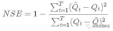
among

Is the average of the observed emissions,

Is the estimated flow at time t, and Qt is the observed flow at time t. NSE values range from − ∞ to 1, where 1 represents perfect prediction performance. A zero NSE indicates that the model has the same prediction performance as the mean of the data set.
nRMSE is a percentage based indicator that describes the difference between predicted and measured emissions:
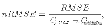
among
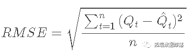
Where Qt is the flow observed at time t,

Is the estimated emission at time t, n is the number of samples,

and

Is the maximum and minimum emissions observed. The resulting nRMSE calculation is a percentage value.
result
site
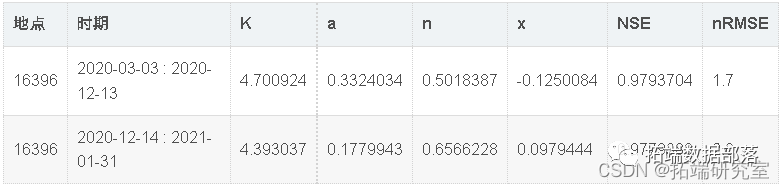
Based on exploratory analysis, two rating curves are developed for the site. The cycle of rating curve is from March 3, 2020 to November 30, 2020 and from December 1, 2020 to January 31, 2021. Due to the obvious unstable flow observed in the water layer, We applied Jones formula (formula (2) "). Both time periods produced rating curves with NSE greater than 0.97 and nRMSE less than 3%, indicating that they are very suitable (Table 2; number 3). Number 3 does indicate that there are some biased flow estimates in very low flow measurement. This is due to the flow changes recorded by Doppler flowmeter at low flow.
## Make a data frame for the site

if %>%
  group_split %>%
  ## Delete events where the maximum flow does not exceed 10 cfs
  imap %>%
  bind_rows
## Create data frames for the site from December 14, 2020 to January 2021
idf %>%
         diff_time %>%
  group_split %>%
  imap(~mutate) %>%
  bind_rows %>%
##Using nls to estimate the parameters in Jones formula
## Some starting parameters. nls_multstart will use multiple
##Start parameter and model selection lookup
##Global minimum
stlower
stupper
##Suitable for nls
rc<- nls(jorm,
suors = "Y")
##Set parameter start limit
##nls
nls(jorm
suors = "Y")## Use the parameter results to set the data frame. It will be used to report parameters and GOF metrics dfresu <- tibble(Site )
## Develop rating curve forecasts and
## Create tables using GOF metrics
df %>%
dfres %>%

 NSE(predicted, as.numeric(Flow))-> dfres

##Display table
kable(dfres)
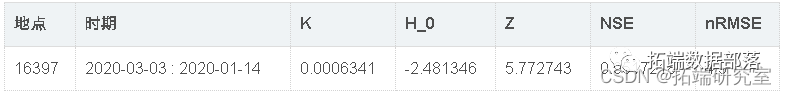
Table 2: site rating curve parameter estimation and goodness of fit indicators
##Draw rating curve results

p1 <- ggplot +
    geom_pointlpha = 0.25) +
  geom_abline +
  scale\_x\_continuous
  theme()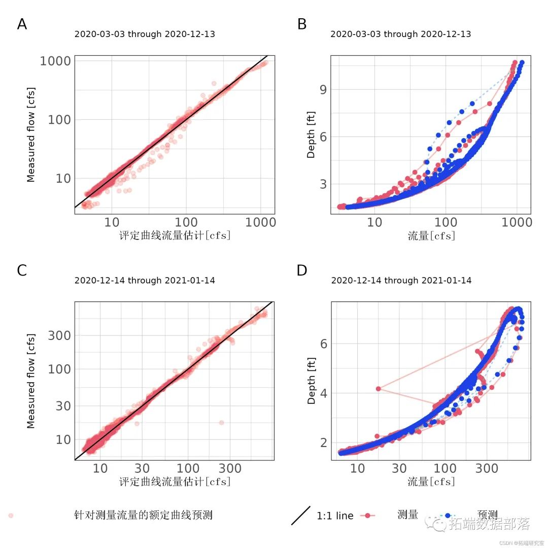
Figure 3: scatter diagram of rated curve estimated flow and measured flow (A, C) and stage flow prediction (B, D) for each rated curve period at the station.
Site 16397
Exploratory analysis shows that, The power function (formula (1) ") is used at this station because no unstable flow conditions are observed in the hydrological process map. The prediction of the rating curve leads to NSE greater than 0.95, indicating that it is very suitable (Table 2). nRMSE is less than 5%, which may be a good result for the small sample size obtained at this station and may be affected by the observed low flow variance (Table 2; Figure 3)
## Set the data frame to fit the rating curve to 1697

##power function

##Parameter start limit

rc_7 <- nls(prm,
              stalower
              supors = "Y")
## Use the parameter results to set the data frame. It will be used later to report parameters and GOF metrics
dfres <- tibble(Sit,
K,
H0 ,
Z\["Z"\]\])df167 %>% mutate(pr = exp(predict(rc))) -> df
Table 3: parameter estimation and goodness of fit index of rating curve at site 167
##Draw rating curve results
p1 <- df7 %>%
   ggplot() +
   geom_point +
   geom_abline+
   scale\_x\_continuous +
   scale\_y\_continuous
p1 + p2 + plot_annotation
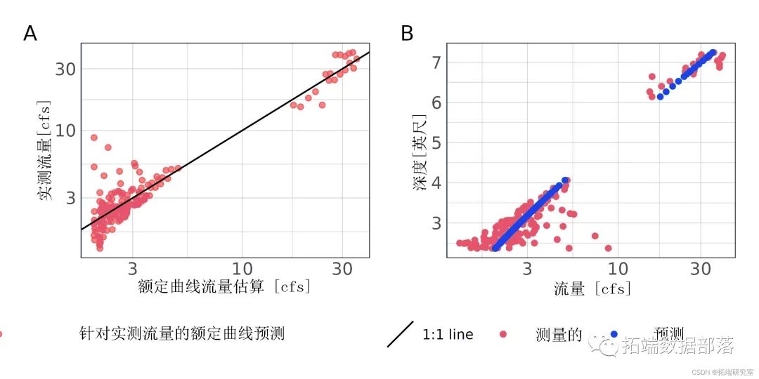
Figure 4: scatter diagram of rated flow, estimated flow and measured flow (A) and stage flow prediction (B) of 167 station.
Site 162
Based on exploratory analysis, three rating curves were developed for site 166. The period of rating curve is from March 3, 2020 to May 30, 2020; From June 1, 2020 to October 31, 2020; And from November 1, 2020 to January 31, 2021. Due to the obvious unstable flow observed in the water layer, We applied the Jones formula (formula (2) "). The results from March to September show that the rating curve has a very good fit (NSE > 0.96, nrmse < 6%; table 4). The large difference between the observed and predicted values at low flow can be attributed to events with extremely fast flow height change (\ > 1.5 ft / h), and the parameter estimation is difficult to fit (Fig. 5). The goodness of fit index of other rating curves decreased, but still showed good performance (Table 4). The high square difference of the measured medium and low flow values affected the performance of the rating curve (Fig. 5)
## Make three different data frames to fit Jones formula.

iqpdf %>%
    filter(DaTime > as.POSIXct)
  #filter %>%
  group_split %>%
  imap %>%
  bind_rows
## Estimate the parameters of each data set
##Set parameter start limit
stlower
stupper
rc<- nls(jonrm
surs = "Y")
##Set parameter start limit
stlower
stupper
rc <- nls(jorm,
stawer,
suprs = "Y")
##Set parameter start limit
stalower## Use the parameter results to set the data frame. It will be used later to report parameters and GOF metrics
dfres <- tibble(Site
K ,
a ,
n ,
x )
## Develop rating curve forecasts and
## Create tables using GOF metrics
##Display table
kable(df)Table 4: parameter estimation and goodness of fit index of rating curve at site 16882

##Draw rating curve results

p1 <- ggplot(df_03) +
    geom_point +
  geom_abline+
  scale\_x\_continuous +
  scale\_y\_continuous +
  theme_ms()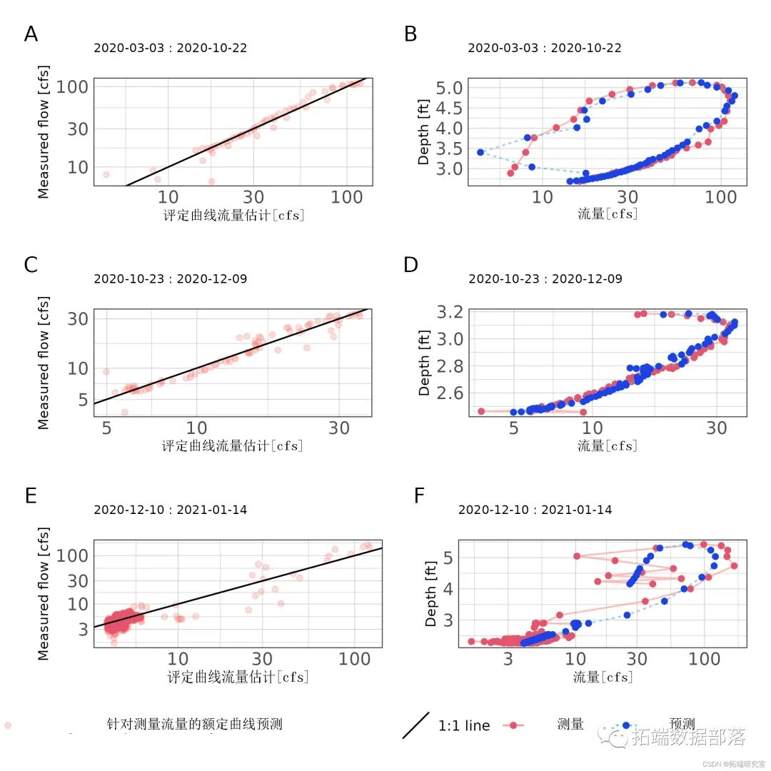
Figure 5: scatter diagram of rated curve estimated flow and measured flow (A, C, E) and stage flow prediction (B, D, F) for each rated curve period of 16882 station.
Daily flow estimation
# Use original dataset
# Estimate flow by date using rating curve
# Aggregation represents daily traffic and reports summary statistics.

hodf %>%
  dplyr::select%>%
  group_split(site) %>%
  bind_rows()

## Make the data frame of the model, predict the data, then map the prediction function, and cancel the nested data frame.
tibble) %>%
    ~exp( newdata = .y))
  )) %>%
  tidyr::unnest%>%
  as_tsibble

##Draw data

ggplot() +
  geom_line+
  geom_point +
  facet_wrap +
  scale\_y\_continuous +
  theme_ms()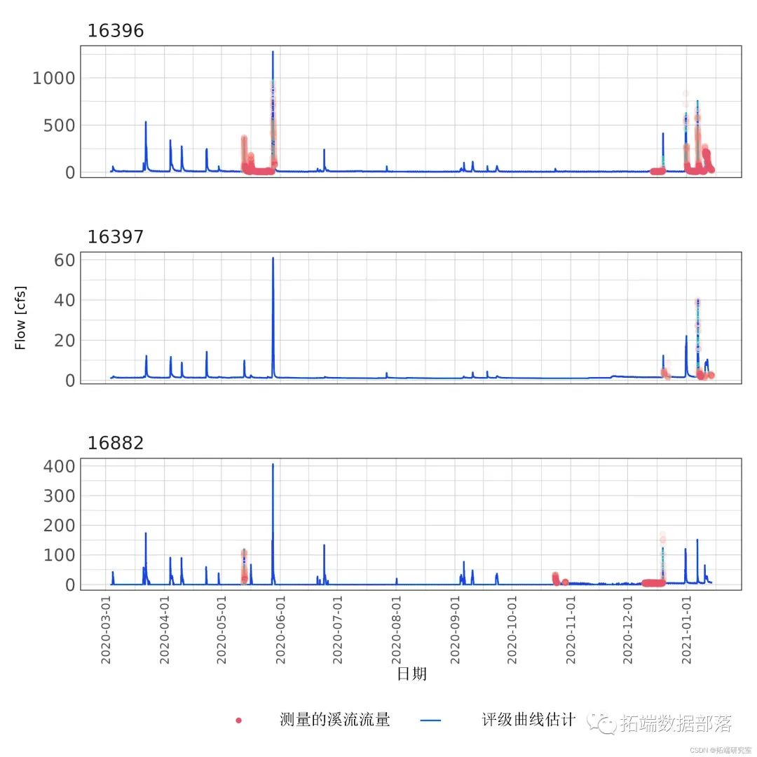
Figure 6: 15 minute flow estimation and superimposed measured flow values
## Calculate average daily traffic and report statistics

   dplyr::select(Site, DTime) %>%
   group\_by\_key() %>%
   index\_by(date = ~as\_date(.)) %>%
## Report summary statistics
meflow %>%
   as_tibble() %>%
   dplyr::select %>%
   tbl_summary %>%
   as_kable()
Table 5: summary statistics of average daily flow estimation of each station

ggplot(mean\_daily\_flow %>% fill_gaps()) +
  geom\_line(aes(date, mean\_daily)) +
  facet\_wrap(~Site, ncol = 1, scales = "free\_y") +
  scale\_x\_date("Date", date_breaks = "1 month",
                   date_labels = "%F") +
  labs(y = "Mean daily streamflow \[cfs\]") +
  theme_ms() +
  guides(x = guide_axis(angle = 90)) +
  theme(axis.text.x = element_text(size = 8))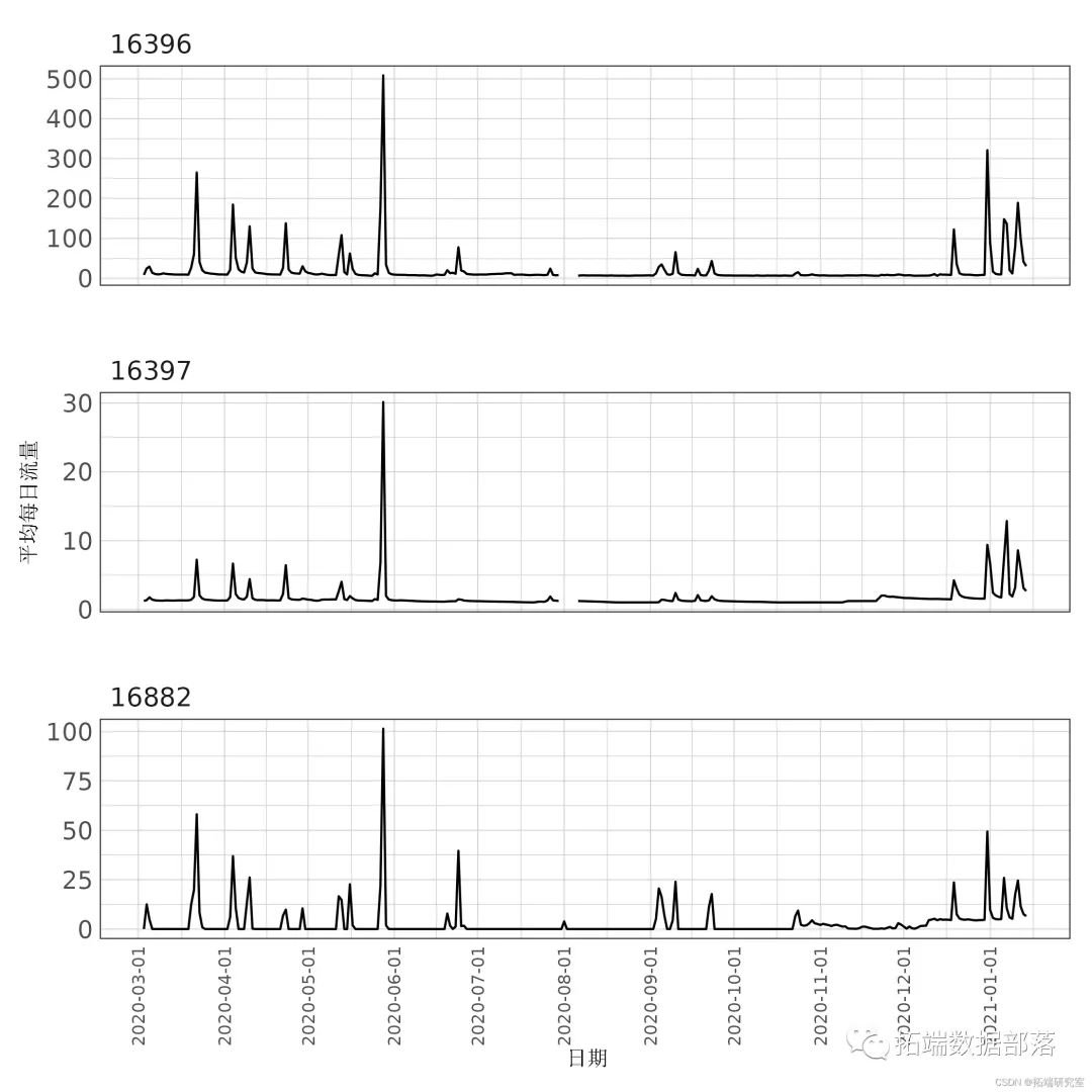
Figure 7: average daily flow estimation.
##Export data
melow %>%
   writcsv("modf.csv")
reference resources
Asquith, William H., Meghan C. Roussel, and Joseph Vrabel. 2006. "Statewide Analysis of the Drainage-Area Ratio Method for 34 Streamflow Percentile Ranges in Texas." 2006-5286. U.S. Geological Survey.
This paper is an excerpt from R language nonlinear regression nls exploration and analysis of river stage flow data, rating curve and flow prediction visualization