Write in front
First of all, I'm lucky to be teammates with Jie Shao and Lin Youxi. It's very easy to play with you. At the same time, I hope my sharing and summary can bring you some help and exchange and study together.

The complete scheme will be presented next!!! Full of dry goods!!!
Dataset download link: https://pan.baidu.com/s/1exjtkUqYPzdWKsCUYGix_g
Extraction code: 0qsm
Game analysis
The title of the competition is "subway passenger flow prediction". By analyzing the historical card swiping data of the subway station, participants can predict the future passenger flow changes of the station, help to realize more reasonable travel route selection, avoid traffic congestion, deploy station security measures in advance, and finally help the safe travel of cities in the future with technologies such as big data and artificial intelligence.
Problem introduction: by analyzing the historical card swiping data of the subway station, predict the incoming and outgoing passenger flow of the station every ten minutes in the future.
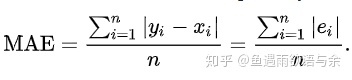
The competition training set includes 25 days of subway card swiping data records from January 1 to January 25. It is divided into three lists: A, B and C. The data records of one day are added respectively to predict the passenger flow in and out of each station every ten minutes in the next day. The evaluation index is MAE.
data set
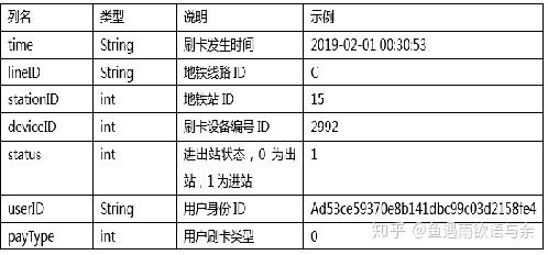
Evaluation index
Difficulty of competition
The competition is divided into three lists. Each list selects different dates, including weeks and weekends. We regard the week as a normal day and the weekend as a special day. How to model these two kinds of dates and how to achieve the maximum prediction accuracy. We summarize the difficulties of this competition as follows.
(1) The label of this competition needs to be built by ourselves. How to model so that we can achieve as much prediction accuracy as possible on a given data set?
(2) The selection of different time periods of the training set has a certain impact on the final results. How to select the time period to make the distribution of the training set similar to that of the test set is also one of the keys of this competition.
(3) How to characterize the timing characteristics of each time period so that it can capture the trend, periodicity and cyclicity of the data set.
(4) There are too many factors affecting the flow of subway stations, such as simultaneous arrival, emergencies, or grand events, so how to deal with outliers to ensure the stability of the model.
In view of the above difficulties, let's explain the idea & details of our team's algorithm design in blocks. Our core idea is mainly divided into three parts: EDA based modeling module, feature engineering module and model training & fusion.
Core idea part1 - EDA based modeling framework
1. Model framework
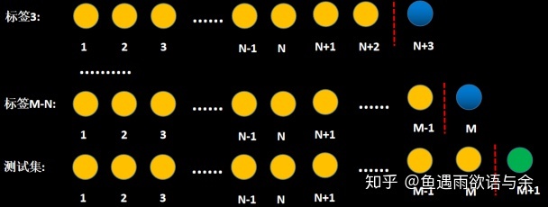
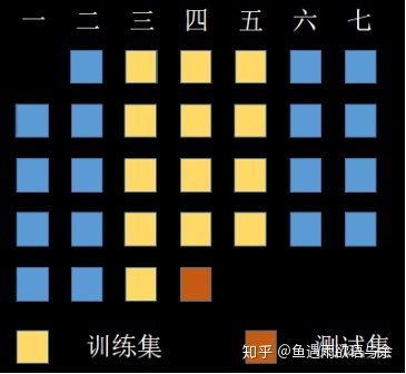
The model is constructed by sliding window rolling (day), which can prevent the model training deviation due to the existence of singular values on a certain day. Finally, the labels and features of all rolling sliding windows are spliced to form our final training set.
Refer to the following figure for the sliding window method:
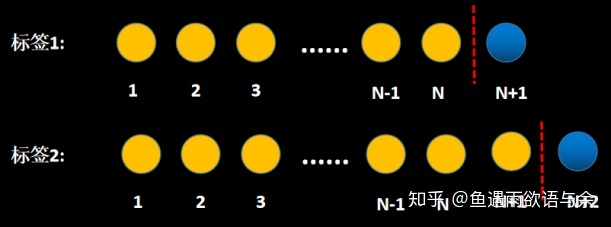
For common timing problems, sampling can be used to extract features and build training sets.
2. Model details
For the sliding window scrolling above, you need to select labels similar to those distributed in the test set to build labels to achieve better results. Therefore, before that, we need to delete data with large distribution differences.
Here we have carried out a simple EDA to analyze the distribution of label. (good EDA can help you understand the data and mine more details, which is essential in the game)
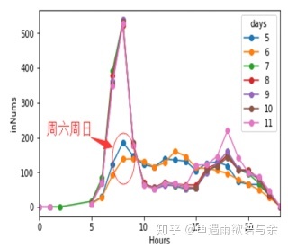
Inbound flow distribution at each time from No. 5 to No. 10
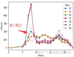
Inbound flow distribution at each time from No. 12 to No. 18
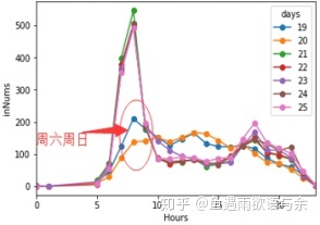
Inbound flow distribution at all times from No. 19 to No. 25
It can be seen from the three figures that there are great differences between weekend and week distribution, so we treat the test set as weekend and test set as week distribution differently to ensure the stability of training set distribution.

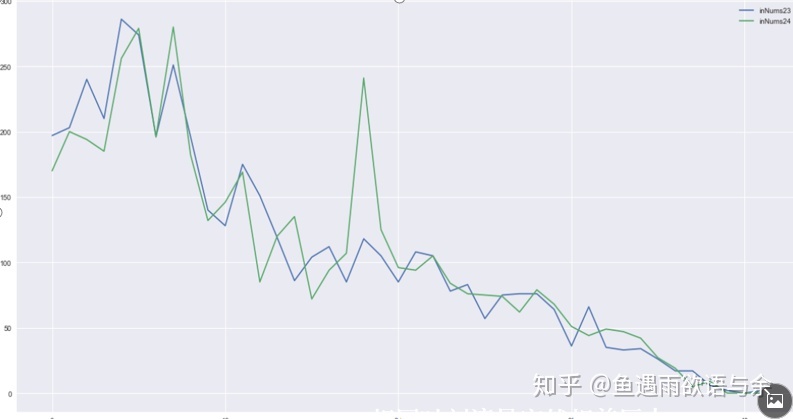
Inbound flow distribution of 23 and 24
It can be seen from the figure that the flow suddenly varies greatly in the same time period. It can be considered because of sudden activities, special events and other factors.
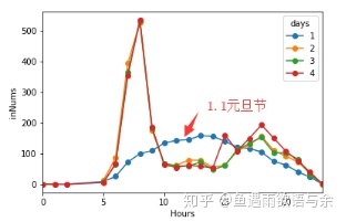
Inbound traffic distribution on New Year's day and the following days
From the distribution of traffic on holidays, we found that the distribution of information on holidays and non holidays is very different, so we also choose to delete it.
Core idea Part2 - Feature Engineering
With the framework of the model, the following is how to describe the flow information of each station at different times. Here, we need to personally think about the factors affecting the flow of subway stations, and think about how to construct relevant features to represent this factor from the available data. Finally, through a large number of EDA and analysis, we construct the characteristics of subway flow through the following modules.

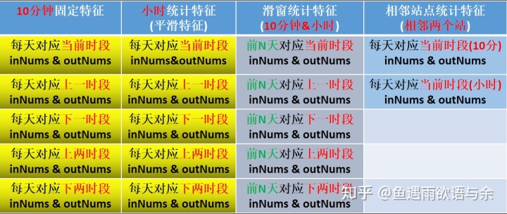
1. Highly relevant information
Strong correlation information mainly occurs at the corresponding time of each day, so we construct hourly and 10 minute inbound and outbound traffic characteristics respectively. Considering the fluctuation factors of the flow in the front and back time periods, the flow characteristics of the previous period and the next period, or the previous two and the next two periods are added. At the same time, the traffic in the corresponding period of the previous N days is also constructed. Further, considering the strong correlation between adjacent stations, the traffic of the corresponding period of two adjacent stations is added.
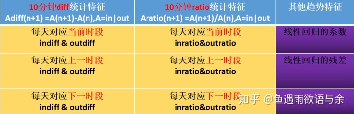
2. Trend
Mining trend is also the key to feature extraction. Our main structural features are defined as follows:

That is, it represents the difference between the previous and subsequent periods. Here, it can be inbound traffic or battle traffic. Similarly, we consider that each day corresponds to the current period, and each day corresponds to the previous period. Of course, we can also consider the difference ratio:

Key codes:
def time_before_trans(x,dic_):
    if x in dic_.keys():
        return dic_[x]
    else:
        return np.nan
def generate_fea_y(df, day, n):
    df_feature_y   =  df.loc[df.days_relative == day].copy()

    df_feature_y['tmp_10_minutes'] = df_feature_y['stationID'].values * 1000 + df_feature_y['ten_minutes_in_day'].values
    df_feature_y['tmp_hours']      = df_feature_y['stationID'].values * 1000 + df_feature_y['hour'].values

    for i in range(n): # Every day of the previous n days
        d = day - i - 1
        df_d = df.loc[df.days_relative == d].copy() # Data of the day

        # Feature 1: how much in and out of this time period (the same time period, 10minutes) in the past
        df_d['tmp_10_minutes'] = df['stationID'] * 1000 + df['ten_minutes_in_day']
        df_d['tmp_hours']      = df['stationID'] * 1000 + df['hour']
        # sum
        dic_innums  = df_d.groupby(['tmp_10_minutes'])['inNums'].sum().to_dict()
        dic_outnums = df_d.groupby(['tmp_10_minutes'])['outNums'].sum().to_dict()
        df_feature_y['_bf_' + str(day -d) + '_innum_10minutes']  =  df_feature_y['tmp_10_minutes'].map(dic_innums).values
        df_feature_y['_bf_' + str(day -d) + '_outnum_10minutes'] =  df_feature_y['tmp_10_minutes'].map(dic_outnums).values

        # Feature 2: how much in and out of this time period (hours) in the past
        dic_innums  = df_d.groupby(['tmp_hours'])['inNums'].sum().to_dict()
        dic_outnums = df_d.groupby(['tmp_hours'])['outNums'].sum().to_dict()
        df_feature_y['_bf_' + str(day -d) + '_innum_hour']  =  df_feature_y['tmp_hours'].map(dic_innums).values
        df_feature_y['_bf_' + str(day -d) + '_outnum_hour'] =  df_feature_y['tmp_hours'].map(dic_outnums).values

        # Feature 3: last 10 minutes
        df_d['tmp_10_minutes_bf'] = df['stationID'] * 1000 + df['ten_minutes_in_day'] - 1
        df_d['tmp_hours_bf']      = df['stationID'] * 1000 + df['hour'] - 1
        # sum
        dic_innums  = df_d.groupby(['tmp_10_minutes_bf'])['inNums'].sum().to_dict()
        dic_outnums = df_d.groupby(['tmp_hours_bf'])['outNums'].sum().to_dict()
        df_feature_y['_bf21_' + str(day -d) + '_innum_10minutes']  =  df_feature_y['tmp_10_minutes'].agg(lambda x: time_before_trans(x,dic_innums)).values
        df_feature_y['_bf1_' + str(day -d) + '_outnum_10minutes'] =  df_feature_y['tmp_10_minutes'].agg(lambda x: time_before_trans(x,dic_outnums)).values

        # Feature 4: last hour
        dic_innums  = df_d.groupby(['tmp_hours_bf'])['inNums'].sum().to_dict()
        dic_outnums = df_d.groupby(['tmp_hours_bf'])['outNums'].sum().to_dict()
        df_feature_y['_bf1_' + str(day -d) + '_innum_hour']  =  df_feature_y['tmp_hours'].map(dic_innums).values
        df_feature_y['_bf1_' + str(day -d) + '_outnum_hour'] =  df_feature_y['tmp_hours'].map(dic_outnums).values


    for col in ['tmp_10_minutes','tmp_hours']:
        del df_feature_y[col]

    return df_feature_y
Add: the above is the code used in the game, but some logic errors were found after the game. This error was not found from list A to list C
# error code
dic_innums  = df_d.groupby(['tmp_10_minutes_bf'])['inNums'].sum().to_dict()
dic_outnums = df_d.groupby(['tmp_hours_bf'])['outNums'].sum().to_dict()
# Modified code
dic_innums  = df_d.groupby(['tmp_10_minutes_bf'])['inNums'].sum().to_dict()
dic_outnums = df_d.groupby(['tmp_10_minutes_bf'])['outNums'].sum().to_dict()
3. Periodicity
Due to the similar distribution of weekends, the distribution of weekdays is similar. Therefore, we select the information corresponding to the date and time period to construct the feature, specifically:

Key codes:
columns = ['_innum_10minutes','_outnum_10minutes','_innum_hour','_outnum_hour']
# # sum,mean in the past n days
for i in range(2,left):
    for f in columns:
        colname1 = '_bf_'+str(i)+'_'+'days'+f+'_sum'
        df_feature_y[colname1] = 0
        for d in range(1,i+1):
            df_feature_y[colname1] = df_feature_y[colname1] + df_feature_y['_bf_'+str(d) +f]
        colname2 = '_bf_'+str(d)+'_'+'days'+f+'_mean'
        df_feature_y[colname2] = df_feature_y[colname1] / i

# Difference of mean in the past n days
for i in range(2,left):
    for f in columns:
        colname1 = '_bf_'+str(d)+'_'+'days'+f+'_mean'
        colname2 = '_bf_'+str(d)+'_'+'days'+f+'_mean_diff'
        df_feature_y[colname2] = df_feature_y[colname1].diff(1)
        df_feature_y.loc[(df_feature_y.hour==0)&(df_feature_y.minute==0), colname2] = 0
4.stationID related features
It is mainly used to mine the heat of different sites and the combination of sites and other features. The key codes are:
def get_stationID_fea(df):
    df_station               = pd.DataFrame()
    df_station['stationID']  = df['stationID'].unique()
    df_station               = df_station.sort_values('stationID')

    tmp1  = df.groupby(['stationID'])['deviceID'].nunique().to_frame('stationID_deviceID_nunique').reset_index()
    tmp2  = df.groupby(['stationID'])['userID'].nunique().to_frame('stationID_userID_nunique').reset_index()

    df_station = df_station.merge(tmp1,on ='stationID', how='left')
    df_station = df_station.merge(tmp2,on ='stationID', how='left')

    for pivot_cols in tqdm_notebook(['payType','hour','days_relative','ten_minutes_in_day']):

        tmp = df.groupby(['stationID',pivot_cols])['deviceID'].count().to_frame('stationID_'+pivot_cols+'_cnt').reset_index()
        df_tmp = tmp.pivot(index = 'stationID', columns=pivot_cols, values='stationID_'+pivot_cols+'_cnt')
        cols   = ['stationID_'+pivot_cols+'_cnt' + str(col) for col in df_tmp.columns]
        df_tmp.columns = cols
        df_tmp.reset_index(inplace = True)
        df_station = df_station.merge(df_tmp, on ='stationID', how='left')
    return df_station
Core idea Part3 - model training & Fusion
In terms of model training, we mainly have three schemes: traditional scheme, smoothing trend and timing stacking. Finally, the predicted results of the three schemes are weighted and fused according to the scores of the offline verification set.
Due to the superiority of the scores of C list, we mainly elaborate the scheme of C list here.
1. Traditional programmes
Since the test set of list C is weekly data, we removed the weekend data to ensure that the distribution is basically consistent. In order to maintain the periodicity of the training set, we removed Monday and Tuesday. This is also modeled as our most basic scheme.
2. Smooth trend
We design a method to deal with singular values, that is, the second scheme is to smooth the trend. The idea of the scheme is that for the days with roughly the same distribution in the week, if the flow fluctuates abnormally at the same time, we define it as singular value. Then select the date with strong correlation with the test set as the benchmark. For example, if the test set in list C is No. 31, select No. 24 as the benchmark to compare the site traffic at the corresponding time of No. 24 and other dates. Here, we construct the trend ratio of traffic on the 24th corresponding to other dates, and modify the traffic for each 10 minutes at the corresponding time according to this trend ratio. Because the hourly flow is more stable, determine the trend ratio according to the hour, and then modify the flow for 10 minutes in the hour. After modifying the traffic, we can model the traditional scheme. Here, we will retain the data of Monday and Tuesday.
Specific steps:
- Delete Saturday and Sunday
- Smooth the time flow trend of the date before the 24th corresponding to the 24th
- Routine training
The key codes of smoothing trend are given below:
if (test_week!=6)&(test_week!=5):
inNums_hour = data[data.day!=31].groupby(['stationID','week','day','hour'])['inNums' ].sum().reset_index(name='inNums_hour_sum')
outNums_hour = data[data.day!=31].groupby(['stationID','week','day','hour'])['outNums'].sum().reset_index(name='outNums_hour_sum')
# Merging neotectonic features
data = data.merge(inNums_hour , on=['stationID','week','day','hour'], how='left')
data = data.merge(outNums_hour, on=['stationID','week','day','hour'], how='left')
data.fillna(0, inplace=True)
# Extract No. 24 flow
test_nums = data.loc[data.day==24, ['stationID','ten_minutes_in_day','inNums_hour_sum','outNums_hour_sum']]
test_nums.columns = ['stationID','ten_minutes_in_day','test_inNums_hour_sum' ,'test_outNums_hour_sum']
# Combined flow 24
data = data.merge(test_nums , on=['stationID','ten_minutes_in_day'], how='left')
# Construct daily and trends
data['test_inNums_hour_trend'] = (data['test_inNums_hour_sum'] + 1) / (data['inNums_hour_sum'] + 1 )
data['test_outNums_hour_trend'] = (data['test_outNums_hour_sum'] + 1) / (data['outNums_hour_sum'] + 1)
if (test_week!=6)&(test_week!=5):
# Initialize new traffic
data['inNums_new'] = data['inNums']
data['outNums_num'] = data['outNums']
for sid in range(0,81):
print('inNums stationID:', sid)
for d in range(2,24):
inNums = data.loc[(data.stationID==sid)&(data.day==d),'inNums']
trend = data.loc[(data.stationID==sid)&(data.day==d),'test_inNums_hour_trend']
data.loc[(data.stationID==sid)&(data.day==d),'inNums_new'] = trend.values*(inNums.values+1)-1
for d in range(25,26):
inNums = data.loc[(data.stationID==sid)&(data.day==d),'inNums']
trend = data.loc[(data.stationID==sid)&(data.day==d),'test_inNums_hour_trend']
data.loc[(data.stationID==sid)&(data.day==d),'inNums_new'] = trend.values*(inNums.values+1)-1
for sid in range(0,81):
print('outNums stationID:', sid)
for d in range(2,24):
outNums = data.loc[(data.stationID==sid)&(data.day==d),'outNums']
trend = data.loc[(data.stationID==sid)&(data.day==d),'test_outNums_hour_trend']
data.loc[(data.stationID==sid)&(data.day==d),'outNums_online'] = trend.values*(outNums.values+1)-1
for d in range(25,26):
outNums = data.loc[(data.stationID==sid)&(data.day==d),'outNums']
trend = data.loc[(data.stationID==sid)&(data.day==d),'test_outNums_hour_trend']
data.loc[(data.stationID==sid)&(data.day==d),'outNums_new'] = trend.values*(outNums.values+1)-1
# Post processing
data.loc[data.inNums_new < 0 , 'inNums_new' ] = 0
data.loc[data.outNums_new < 0 , 'outNums_new'] = 0
data['inNums'] = data['inNums_new']
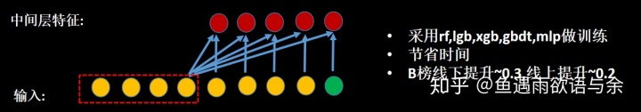
data['outNums'] = data['outNums_new']3. Timing Stacking
Because there are some unknown singular values in the historical data, for example, some large-scale activities will increase the traffic of some stations at some times, and these data have a great impact. In order to reduce the impact of such data, we use the method of time series stacking. If the model prediction results are quite different from our real results, such data is abnormal, The visualization of the scheme is as follows. Through the following operations, we can steadily improve offline and online.
4. Model fusion

The three schemes have their own advantages, and the correlation of offline performance is also low. After fusion, the offline results are more stable. Finally, we weighted them according to the performance of offline CV s.
Experimental results Part4
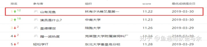
The result of ranking A is the first

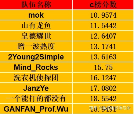
Second place in BC list
In the above code, we won the first place in the A list online. We can also get the second place by removing the failed team from the BC list.
Summary of competition experience
1. The model has strong robustness, ranking first in A list and second in BC list
2. A method to deal with singular values is designed, and a consistent improvement is achieved on the line and off the line
3. Relatively complete time series feature engineering + data selection in different periods