1, Heston option pricing model theory

The birth of BS option pricing model in 1973 marked that option pricing entered the stage of accurate quantitative measurement. However, BS model assumes that the volatility of the underlying asset is constant, which is seriously inconsistent with the "volatility smile" curve observed in the real market.
heston assumes that the price of the underlying asset follows the following process, in which the volatility is a time-varying function [1]:

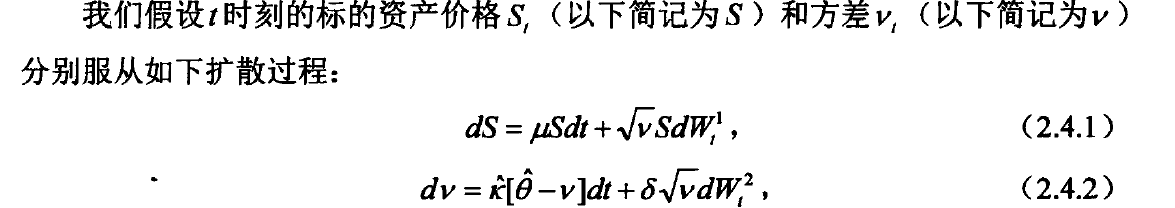
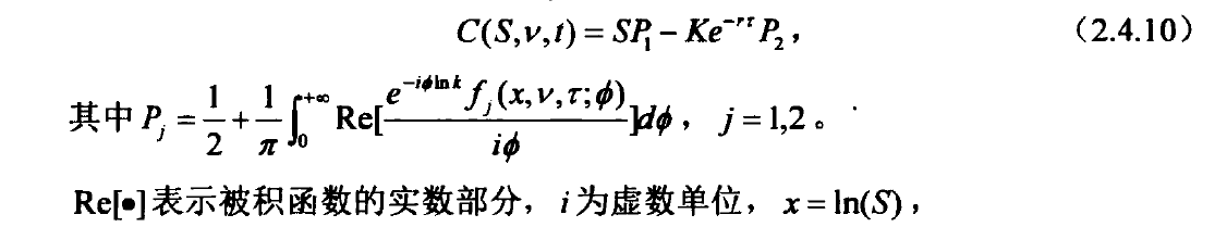
And the European call option pricing formula [2] is obtained:


This paper uses python to implement the above pricing formula. A total of nine parameters need to be input into the formula, of which [v0,kappa,theta,sigma,rho] needs to be set and filled in by yourself in advance. The other four [K,t,s0,r]: [strike price, remaining time, underlying asset price, risk-free interest rate] are option price data. These parameters are also required for BS model pricing.

2, python code for Heston option pricing

The code directory used in this article is shown in the following figure. These documents play their respective roles and together form the whole project. The functions of each file will be described one by one below. You can download the project compressed package from Baidu cloud address and decompress it to view the following files. Baidu cloud disk address: link: https://pan.baidu.com/s/1y7SKSub5gcDD7ZEnmAUUmw
Extraction code: fevc

1. Heston call option price calculation py

This document is mainly used to calculate the Heston call option price. Nine parameters need to be input into the model, among which the execution price K, the remaining maturity time (year) t, the underlying asset price s0 and the risk-free rate of return r are the original sample data that can be obtained from the market; The other five parameters v0, kappa, theta, sigma and rho cannot be obtained from the market, so they need to be specified in advance. Default values have been specified in advance in this article. As shown at the end of the file, the usage of the file is as follows:

if __name__=='__main__':
    #Try to calculate the heston price of a European call option, in which the strike price is 2.15, the remaining maturity is 0.05924 years, the underlying asset price is 2.143896, and the risk-free return is 3.043%
    HC=HestonCall(K =2.15, t = 0.05924, s0 = 2.143896, r = 0.03043)
    HC.Call_Value()#It is found that the calculated price is 0.02445730985668737

2. Simulated annealing algorithm py

This is a general simulated annealing algorithm class, which can be used to solve the function maximization problem. As shown at the end of the file, the specific usage is as follows:

if __name__=='__main__':
    # Use the simulated return algorithm to solve the minimum value of the following function
    def func_target(list_x):
        x1 = list_x[0]
        x2 = list_x[1]
        return 3 * (x1 - 5) ** 2 + 6 * (x2 - 6) ** 2 - 7

    ng=NG(func=func_target,x0=[8,9])
    ng.run()
    x,f=ng.get_history_best_xy()#View historical best solution
    ng.plot_best()#Draw the change process of the optimal solution

3. Simulated annealing algorithm for solving Heston model parameters py

This is an auxiliary function file, which is equivalent to building a bridge between the above two files.

4. Used to control the value range of random number py

This is a supporting document. Because the simulated annealing algorithm may produce unreasonable random numbers in the running process. Therefore, with this file, the generated random number is limited to the specified range, so as to prevent too extreme numbers from damaging the operation of the algorithm.
As shown at the end of the file, the specific usage is as follows:

    x=0.3;a=0;b=4
    sum_False=0
    x_all=[]
    for i in range(1000):
        x=random_range(x,a,b)
        x_all.append(x)
        print(x)
        if x>b or x<a:
            sum_False+=1

5. Solve the Heston optimal parameter estimation py

This is a summary file, which is equivalent to collecting the files of other functions in one place and using the algorithm to calculate the optimal parameters.

3, Specific use method and training process

The user only needs to open main Py file by modifying date_start_train and date_end_train to select the sample data within the specified time range (note that the time range should not exceed the sample data range), and then run the whole file. As shown at the end of the file, the specific usage is as follows:

if __name__=='__main__':
    data = pd.read_csv('SSE 50 ETF Option data.csv')  # Read raw data

    date_start_train = 20200912#Select the start date of the data
    date_end_train = 20201212#Select the end date of the data
    option = data[(data['Transaction date'] >= date_start_train) & (data['Transaction date'] <= date_start_train)]#Select the data within the specified time range

    option = option[option['Bullish and bearish types'] == 'C']#Select call option data
    option = option[['Execution price', 'Remaining maturity (years)', 'SSE 50 ETF Price', 'Risk free rate of return( shibor)', 'Option closing price']]#Select the data you want to use
    option.columns = ['K', 't', 's0', 'r', 'c']#Change the column header name to a format that you can use

    model = SV_SA(data=option)#Create class
    model.sa()#Start training data
    model.ng.get_history_best_xy()#View the best parameters for your workout

If the function works normally, it means that the model begins to train. As shown in the figure below:

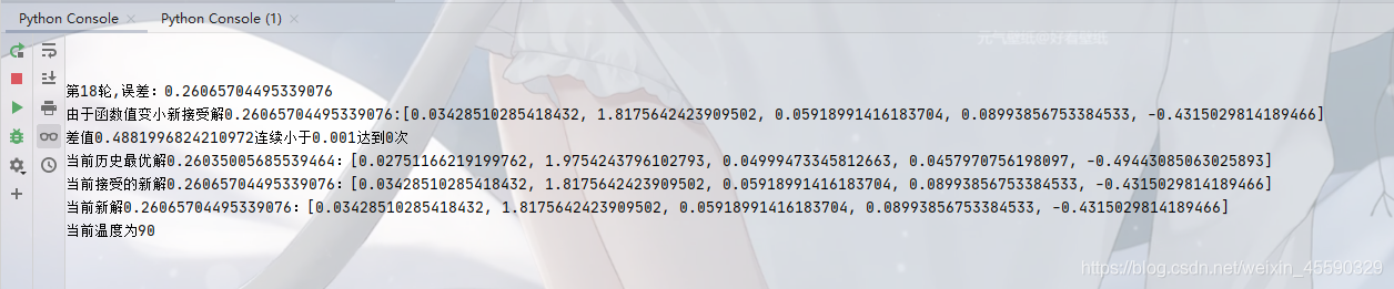
The longer the selected time range, the more data, the longer the training time, and you need to wait patiently. The 18th round on the first line in the figure shows that it has been trained 18 times.
The 0.26065704495339076 in the fourth line indicates that after so many rounds of training, the minimum mean error was once this number. The following [0.03428510285418432, 1.817564242399502, 0.05918991416183704, 0.08993856753384533, -0.43150298189466] indicates that the current optimal solution should be this number, that is, the optimal value estimated by the last five parameters of heston model.
Theoretically, with the passage of time, such as training day and night, the training error in the fourth line will become smaller and smaller, the smaller the better. However, if the model training does not stop, you can also select the five current optimal solutions after the fourth line as the target value.