Original link: http://tecdat.cn/?p=6714
Original source: Tuo end data tribal official account
It is common that image classification models must be trained with very little data, which may be encountered in practice if you conduct computer vision in a professional environment. "Few" samples can represent anywhere from hundreds to tens of thousands of images. As a practical example, we will focus on the dataset that classifies images into dogs or cats, which contains 4000 cat and dog images (2000 cats, 2000 dogs). We will use 2000 images for training - 1000 for verification and 1000 for testing.
Correlation between deep learning and small data problems
You sometimes hear that deep learning is only effective when a large amount of data is available. This part is effective: a basic feature of deep learning is that it can find interesting features in the training data without manual feature engineering, which can be realized only when a large number of training examples are available. This is especially true for problems with very high dimensions of input samples, such as images.
Let's start with the data.
Download data
Use the Dogs vs. Cats dataset.
Here are some examples:
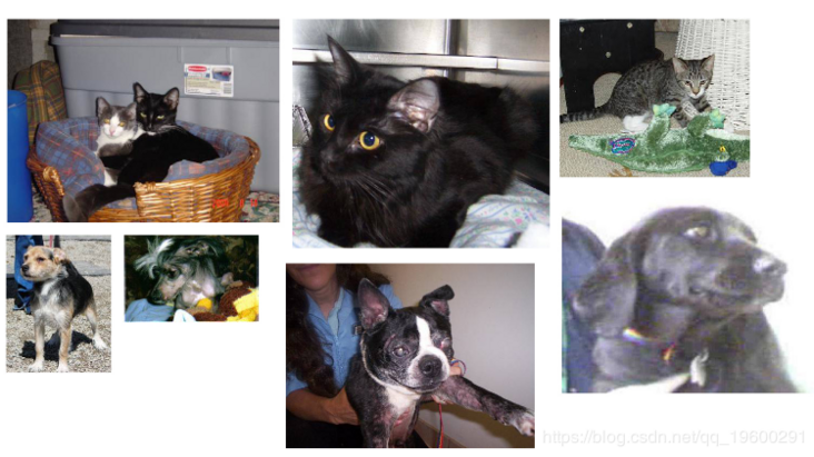
The data set contains 25000 images of dogs and cats (12500 images per class) and 543 MB. After downloading and decompressing, you will create a new data set with three subsets: a training set with 1000 samples per class, a validation set with 500 samples per class, and a test set with 500 samples per class.
Here is the code to do this:
original\_dataset\_dir < - "〜/ Downloads / kaggle\_original\_data"
base\_dir < - "〜/ Downloads / cats\_and\_dogs\_small"dir.create(base_dir)
train\_dir < -  file.path(base\_dir,"train")
dir.create(train_dir)
validation\_dir < -  file.  path(base\_dir,"validation")
Using pre trained convnet
A common and efficient method of in-depth learning on small image data sets is to use pre training network. A pre trained network is a saved network previously trained on large data sets, usually on large-scale image classification tasks. If the original data set is large enough and general enough, the spatial hierarchy of the features of the pre training network learning can effectively act as a general model of the visual world. Therefore, its features can prove useful for many different computer vision problems, even though these new problems may involve classes completely different from the original task.
There are two ways to use the pre training network: feature extraction and fine tuning. Let's start with feature extraction.
feature extraction
Feature extraction includes extracting features of interest from new samples using the representation of previous network learning. These functions will then be run through a new classifier, which is trained from scratch.
Why reuse only convolution cardinality? Can you reuse densely connected classifiers? In general, this should be avoided. The reason is that the representation of convolution based learning may be more general and therefore more reusable.
be careful, The level of generality (and therefore reusability) of the representation extracted by a particular convolution layer depends on the depth of the layer in the model. Earlier layers in the model extract local, highly generic feature maps (such as visual edges, colors and textures), while higher layers extract more abstract concepts (such as "cat ears" or "dog eyes") ) . Therefore, if your new data set is very different from the data set training the original model, it is best to use only the first few layers of the model for feature extraction, rather than the whole convolution basis.
Let's achieve this by using the convolution basis of VGG16 network trained on ImageNet, extract interesting features from cat and dog images, and then train dog and cat classifiers on these features.
Let's instantiate the VGG16 model.
conv\_base < - application\_vgg16(weights ="imagenet",include\_top = FALSE,input\_shape = c(150,150,3))
Pass three parameters to the function:
- Weights specifies the weights from which to initialize the model.
- include_top "dense connection" refers to the classifier that includes (or does not include) dense connections at the top of the network. By default, this dense connection classifier corresponds to 1000 classes of ImageNet.
- input_shape is the shape of the image tensor that you will provide to the network. This parameter is optional: if you don't pass it, the network will be able to handle input of any size.
It is similar to the simple network you are already familiar with:
summary(conv_base)

Layer (type)                     Output Shape          Param #
================================================================
input_1 (InputLayer)             (None, 150, 150, 3)   0
\_\_\_\_\_\_\_\_\_\_\_\_\_\_\_\_\_\_\_\_\_\_\_\_\_\_\_\_\_\_\_\_\_\_\_\_\_\_\_\_\_\_\_\_\_\_\_\_\_\_\_\_\_\_\_\_\_\_\_\_\_\_\_\_
block1_conv1 (Convolution2D)     (None, 150, 150, 64)  1792
\_\_\_\_\_\_\_\_\_\_\_\_\_\_\_\_\_\_\_\_\_\_\_\_\_\_\_\_\_\_\_\_\_\_\_\_\_\_\_\_\_\_\_\_\_\_\_\_\_\_\_\_\_\_\_\_\_\_\_\_\_\_\_\_
block1_conv2 (Convolution2D)     (None, 150, 150, 64)  36928
\_\_\_\_\_\_\_\_\_\_\_\_\_\_\_\_\_\_\_\_\_\_\_\_\_\_\_\_\_\_\_\_\_\_\_\_\_\_\_\_\_\_\_\_\_\_\_\_\_\_\_\_\_\_\_\_\_\_\_\_\_\_\_\_
block1_pool (MaxPooling2D)       (None, 75, 75, 64)    0
\_\_\_\_\_\_\_\_\_\_\_\_\_\_\_\_\_\_\_\_\_\_\_\_\_\_\_\_\_\_\_\_\_\_\_\_\_\_\_\_\_\_\_\_\_\_\_\_\_\_\_\_\_\_\_\_\_\_\_\_\_\_\_\_
block2_conv1 (Convolution2D)     (None, 75, 75, 128)   73856
\_\_\_\_\_\_\_\_\_\_\_\_\_\_\_\_\_\_\_\_\_\_\_\_\_\_\_\_\_\_\_\_\_\_\_\_\_\_\_\_\_\_\_\_\_\_\_\_\_\_\_\_\_\_\_\_\_\_\_\_\_\_\_\_
block2_conv2 (Convolution2D)     (None, 75, 75, 128)   147584
\_\_\_\_\_\_\_\_\_\_\_\_\_\_\_\_\_\_\_\_\_\_\_\_\_\_\_\_\_\_\_\_\_\_\_\_\_\_\_\_\_\_\_\_\_\_\_\_\_\_\_\_\_\_\_\_\_\_\_\_\_\_\_\_
block2_pool (MaxPooling2D)       (None, 37, 37, 128)   0
\_\_\_\_\_\_\_\_\_\_\_\_\_\_\_\_\_\_\_\_\_\_\_\_\_\_\_\_\_\_\_\_\_\_\_\_\_\_\_\_\_\_\_\_\_\_\_\_\_\_\_\_\_\_\_\_\_\_\_\_\_\_\_\_
block3_conv1 (Convolution2D)     (None, 37, 37, 256)   295168
\_\_\_\_\_\_\_\_\_\_\_\_\_\_\_\_\_\_\_\_\_\_\_\_\_\_\_\_\_\_\_\_\_\_\_\_\_\_\_\_\_\_\_\_\_\_\_\_\_\_\_\_\_\_\_\_\_\_\_\_\_\_\_\_
block3_conv2 (Convolution2D)     (None, 37, 37, 256)   590080
\_\_\_\_\_\_\_\_\_\_\_\_\_\_\_\_\_\_\_\_\_\_\_\_\_\_\_\_\_\_\_\_\_\_\_\_\_\_\_\_\_\_\_\_\_\_\_\_\_\_\_\_\_\_\_\_\_\_\_\_\_\_\_\_
block3_conv3 (Convolution2D)     (None, 37, 37, 256)   590080
\_\_\_\_\_\_\_\_\_\_\_\_\_\_\_\_\_\_\_\_\_\_\_\_\_\_\_\_\_\_\_\_\_\_\_\_\_\_\_\_\_\_\_\_\_\_\_\_\_\_\_\_\_\_\_\_\_\_\_\_\_\_\_\_
block3_pool (MaxPooling2D)       (None, 18, 18, 256)   0
\_\_\_\_\_\_\_\_\_\_\_\_\_\_\_\_\_\_\_\_\_\_\_\_\_\_\_\_\_\_\_\_\_\_\_\_\_\_\_\_\_\_\_\_\_\_\_\_\_\_\_\_\_\_\_\_\_\_\_\_\_\_\_\_
block4_conv1 (Convolution2D)     (None, 18, 18, 512)   1180160
\_\_\_\_\_\_\_\_\_\_\_\_\_\_\_\_\_\_\_\_\_\_\_\_\_\_\_\_\_\_\_\_\_\_\_\_\_\_\_\_\_\_\_\_\_\_\_\_\_\_\_\_\_\_\_\_\_\_\_\_\_\_\_\_
block4_conv2 (Convolution2D)     (None, 18, 18, 512)   2359808
\_\_\_\_\_\_\_\_\_\_\_\_\_\_\_\_\_\_\_\_\_\_\_\_\_\_\_\_\_\_\_\_\_\_\_\_\_\_\_\_\_\_\_\_\_\_\_\_\_\_\_\_\_\_\_\_\_\_\_\_\_\_\_\_
block4_conv3 (Convolution2D)     (None, 18, 18, 512)   2359808
\_\_\_\_\_\_\_\_\_\_\_\_\_\_\_\_\_\_\_\_\_\_\_\_\_\_\_\_\_\_\_\_\_\_\_\_\_\_\_\_\_\_\_\_\_\_\_\_\_\_\_\_\_\_\_\_\_\_\_\_\_\_\_\_
block4_pool (MaxPooling2D)       (None, 9, 9, 512)     0
\_\_\_\_\_\_\_\_\_\_\_\_\_\_\_\_\_\_\_\_\_\_\_\_\_\_\_\_\_\_\_\_\_\_\_\_\_\_\_\_\_\_\_\_\_\_\_\_\_\_\_\_\_\_\_\_\_\_\_\_\_\_\_\_
block5_conv1 (Convolution2D)     (None, 9, 9, 512)     2359808
\_\_\_\_\_\_\_\_\_\_\_\_\_\_\_\_\_\_\_\_\_\_\_\_\_\_\_\_\_\_\_\_\_\_\_\_\_\_\_\_\_\_\_\_\_\_\_\_\_\_\_\_\_\_\_\_\_\_\_\_\_\_\_\_
block5_conv2 (Convolution2D)     (None, 9, 9, 512)     2359808
\_\_\_\_\_\_\_\_\_\_\_\_\_\_\_\_\_\_\_\_\_\_\_\_\_\_\_\_\_\_\_\_\_\_\_\_\_\_\_\_\_\_\_\_\_\_\_\_\_\_\_\_\_\_\_\_\_\_\_\_\_\_\_\_
block5_conv3 (Convolution2D)     (None, 9, 9, 512)     2359808
\_\_\_\_\_\_\_\_\_\_\_\_\_\_\_\_\_\_\_\_\_\_\_\_\_\_\_\_\_\_\_\_\_\_\_\_\_\_\_\_\_\_\_\_\_\_\_\_\_\_\_\_\_\_\_\_\_\_\_\_\_\_\_\_
block5_pool (MaxPooling2D)       (None, 4, 4, 512)     0
================================================================
Total params: 14,714,688
Trainable params: 14,714,688
Non-trainable params: 0
At this point, there are two ways to continue:
- Run convolution on the dataset.
- conv_base extends your model () by adding dense layers at the top.
In this article, we will introduce the second technology in detail. Note that you should only try if you can access the GPU.
Feature extraction
Because a model behaves like a layer, you can add a model, such as conv_base, to a sequential model just as you add a layer.
model < - keras\_model\_sequential()%>%conv\_base%>%layer\_flatten()%>%layer\_dense( = 256,activation ="relu")%>%layer\_dense(u its = , "sigmoid")
This is what the model looks like now:
summary(model)

Layer (type)                     Output Shape          Param #
================================================================
vgg16 (Model)                    (None, 4, 4, 512)     14714688
\_\_\_\_\_\_\_\_\_\_\_\_\_\_\_\_\_\_\_\_\_\_\_\_\_\_\_\_\_\_\_\_\_\_\_\_\_\_\_\_\_\_\_\_\_\_\_\_\_\_\_\_\_\_\_\_\_\_\_\_\_\_\_\_
flatten_1 (Flatten)              (None, 8192)          0
\_\_\_\_\_\_\_\_\_\_\_\_\_\_\_\_\_\_\_\_\_\_\_\_\_\_\_\_\_\_\_\_\_\_\_\_\_\_\_\_\_\_\_\_\_\_\_\_\_\_\_\_\_\_\_\_\_\_\_\_\_\_\_\_
dense_1 (Dense)                  (None, 256)           2097408
\_\_\_\_\_\_\_\_\_\_\_\_\_\_\_\_\_\_\_\_\_\_\_\_\_\_\_\_\_\_\_\_\_\_\_\_\_\_\_\_\_\_\_\_\_\_\_\_\_\_\_\_\_\_\_\_\_\_\_\_\_\_\_\_
dense_2 (Dense)                  (None, 1)             257
================================================================
Total params: 16,812,353
Trainable params: 16,812,353
Non-trainable params: 0
As you can see, the convolution cardinality of VGG16 has 14714688 parameters, which is very large.
In Keras, use the following freeze_ The weights() function freezes the network:
freeze\_weights(conv\_base)
length(model $ trainable_weights)
Using data expansion
Overfitting is due to too many samples to learn, resulting in the inability to train models that can be extended to new data.
In Keras, this can be done by configuring multiple random transformations performed on the read image, image\_data\_generator(). For example:
train\_datagen = image\_data\_generator(rescale = 1/255, = 40,width\_shift\_range = 0.2,height\_shift\_range = 0.2, = 0.2,zoom\_range = 0.2,horizo = TRUE,fill_mode ="nearest")
Take a look at this Code:
- rotation_range is a value of degrees (0-180), a range of randomly rotated pictures.
- width\_shift and height\_shift is the range that randomly shifts the picture in a vertical or horizontal direction.
- shear_range is used to randomly apply the shear transform.
- zoom_range is used to randomly scale the inside of a picture.
- horizontal_flip is used to randomly flip half the image horizontally - relevant when there is no horizontal asymmetry assumption (e.g., real-world images).
- fill_mode is a strategy for filling newly created pixels and can appear after rotation or width / height offset.
Now we can train our model using the image data generator:
model%>%compile(loss ="binary\_crossentropy",optimizer = optimizer\_rmsprop(lr = 2e-5),metrics = c("accuracy"))
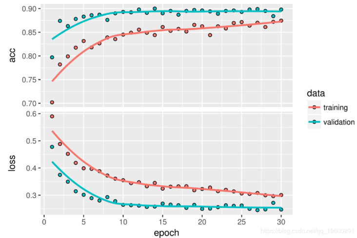
history < - model%>%fit\_generator(train\_generator,steps\_per\_epoch = 100,Draw the results. The accuracy is about 90%.
Fine tuning
Another widely used model reuse technology is a supplement to feature extraction. It is fine-tuning. The steps of fine-tuning the network are as follows:
- Add a custom network to the trained basic network.
- Freeze the underlying network.
- Train the part you added.
- Thaw some layers in the underlying network.
- Jointly train these layers and the parts you add.
You have completed the first three steps in feature extraction. Let's continue with step 4: you'll unfreeze your content conv_base, and then freeze the layers in it.
Now you can start fine tuning the network.
model%>%compile(lo ropy",optimizer = opt imizer_rmsprop(lr = 1e-5),metrics = c("accuracy"))
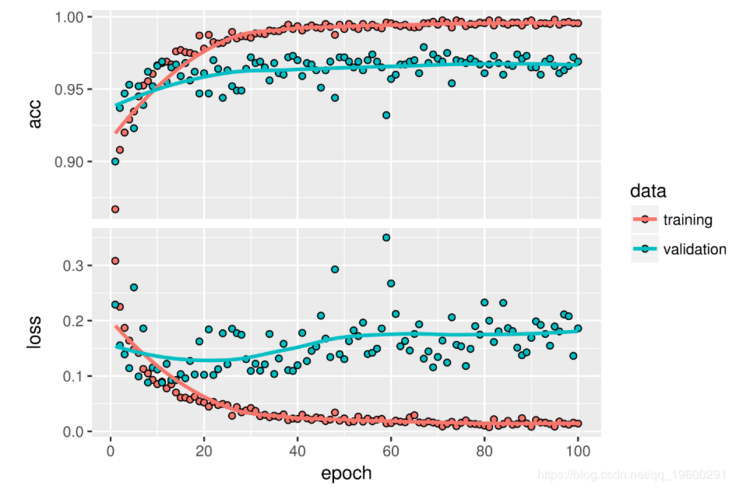
his el%>%fit\_generator(train\_ g steps\_per\_epoch = 100,epochs = 100 ,validation\_data = validation\_genera tor,validation_steps = 50)Let's plot the results:
·
You can see a 6% improvement in accuracy, from about 90% to more than 96%.
You can now finally evaluate this model on test data:
test\_generator < -   (test\_dir,test\_datagen,target\_size = c(150,150),batch_size = 20,  ="binary")

model%>%evaluate_generator( ,steps = 50)
$ loss

\[1\] 0.2158171


$ acc

\[1\] 0.965
Here, you can get 96.5% test accuracy.