anomaly detection

reference material: https://github.com/fengdu78/Coursera-ML-AndrewNg-Notes
Look at the data first:

import numpy as np
import matplotlib.pyplot as plt
from scipy import stats
from scipy.io import loadmat
import math
data = loadmat('data/ex8data1.mat')  # Xval,yval,X
X = data['X']
Xval = data['Xval']
yval = data['yval']
plt.scatter(X[:,0], X[:,1])
plt.show()

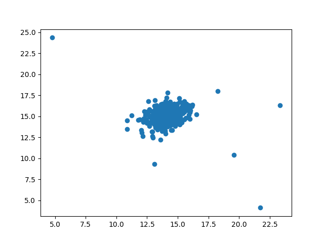
Several points are obviously off center and should be abnormal data points. Let's let the machine learn to detect these abnormal data points:
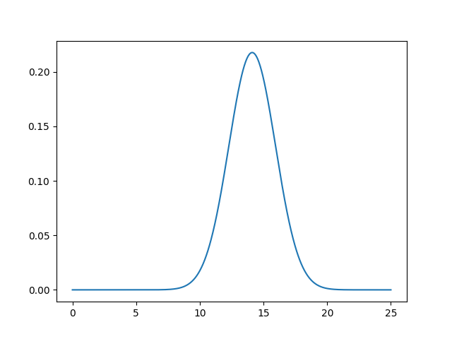
Firstly, two Gaussian functions are established according to two characteristics:

def estimate_gaussian(X):
    mu = X.mean(axis=0)  # 10. Mean() takes the mean value of all data, and X.mean(axis=0) takes the mean value of all columns
    sigma = X.var(axis=0)  # variance
    return mu, sigma


mu, sigma = estimate_gaussian(X)  # X mean (mu) and variance (sigma) of each feature


p = np.zeros((X.shape[0], X.shape[1]))  # X.shape = (307,2)
p0 = stats.norm(mu[0], sigma[0])
p1 = stats.norm(mu[1], sigma[1])
p[:,0] = p0.pdf(X[:,0])
p[:,1] = p1.pdf(X[:,1])

stats.norm automatically creates a Gaussian distribution function (normal distribution) according to the incoming mean and variance, and p0.pdf(x) brings x into the established Gaussian distribution function to get the output.
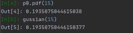
For the sake of rigor, the author manually created a function of Gaussian distribution:

def gussian(x,mu=mu[0], sigma=sigma[0]):
    s = 1/(math.sqrt(2*math.pi)*sigma)
    ss = np.exp(-1*(np.power((x-mu),2))/(2*np.power(sigma,2)))
    return s*ss

The result can not be said to be exactly the same, it can also be said to be exactly the same. (Note: because there are two characteristics, there are two Gaussian functions. Only one example is drawn here)

According to the following function, the best threshold is found through the verification set and F1 (the trade-off between precision and recall can be referred to Wu Enda's study notes v5.51166 ~ 168)

def select_threshold(pval, yval):
    best_epsilon = 0
    best_f1 = 0

    step = (pval.max() - pval.min()) / 1000

    for epsilon in np.arange(pval.min(), pval.max(), step):
        preds = pval < epsilon
        #  np.logical_and logic and
        tp = np.sum(np.logical_and(preds == 1, yval == 1)).astype(float)
        fp = np.sum(np.logical_and(preds == 1, yval == 0)).astype(float)
        fn = np.sum(np.logical_and(preds == 0, yval == 1)).astype(float)

        precision = tp / (tp + fp)
        recall = tp / (tp + fn)
        f1 = (2 * precision * recall) / (precision + recall)

        if f1 > best_f1:
            best_f1 = f1
            best_epsilon = epsilon

    return best_epsilon, best_f1

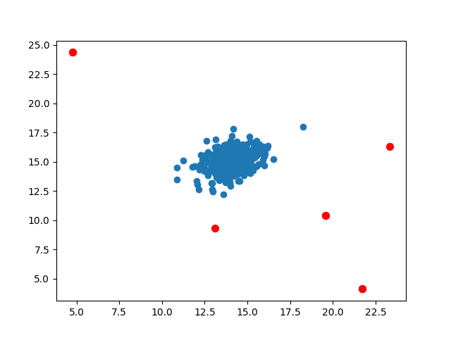
Then it is easy to distinguish the abnormal data. Bring X into the two established Gaussian functions to obtain the abnormal probability, find the data less than the threshold, mark and complete

p = np.zeros((X.shape[0], X.shape[1]))  # X.shape = (307,2)
p0 = stats.norm(mu[0], sigma[0])
p1 = stats.norm(mu[1], sigma[1])
p[:,0] = p0.pdf(X[:,0])
p[:,1] = p1.pdf(X[:,1])


pval = np.zeros((Xval.shape[0], Xval.shape[1]))  # Xval.shape = (307,2)
pval[:,0] = stats.norm(mu[0], sigma[0]).pdf(Xval[:,0])  # Column 0 of pval is the first feature of the verification set, and the Gaussian function value established according to the first feature of X is brought in
pval[:,1] = stats.norm(mu[1], sigma[1]).pdf(Xval[:,1])
epsilon, f1 = select_threshold(pval, yval)  # The optimal threshold is obtained by pval, and then the threshold epsilon is used to find the abnormal value in p
outliers = np.where(p < epsilon)
plt.scatter(X[:,0], X[:,1])
plt.scatter(X[outliers[0],0], X[outliers[0],1], s=50, color='r', marker='o')
plt.show()

When predicting new data, the mean and variance of the two features and their thresholds can be saved, the Gaussian distribution function can be constructed in the new code, and the new features can bring in anomalies less than the threshold.

Collaborative filtering

That is, the recommendation system. It's too difficult for me. This one took a long time. Someone who can think of this algorithm

The code is as follows:

import numpy as np
import scipy.optimize as opt
from scipy.io import loadmat


def serialize(X, theta):  # Develop into one-dimensional reconnection
    return np.concatenate((X.ravel(), theta.ravel()))


def deserialize(param, n_movie, n_user, n_features):  # Then reshape into a vector
    """into ndarray of X(1682, 10), theta(943, 10)"""
    return param[:n_movie * n_features].reshape(n_movie, n_features), \
           param[n_movie * n_features:].reshape(n_user, n_features)


def cost(param, Y, R, n_features):
    """compute cost for every r(i, j)=1
    Args:
        param: serialized X, theta
        Y (movie, user), (1682, 943): (movie, user) rating
        R (movie, user), (1682, 943): (movie, user) has rating
    """
    # theta (user, feature), (943, 10): user preference
    # X (movie, feature), (1682, 10): movie features
    n_movie, n_user = Y.shape
    X, theta = deserialize(param, n_movie, n_user, n_features)

    inner = np.multiply(X @ theta.T - Y, R)

    return np.power(inner, 2).sum() / 2


def gradient(param, Y, R, n_features):
    # theta (user, feature), (943, 10): user preference
    # X (movie, feature), (1682, 10): movie features
    n_movies, n_user = Y.shape
    X, theta = deserialize(param, n_movies, n_user, n_features)

    inner = np.multiply(X @ theta.T - Y, R)  # (1682, 943)

    # X_grad (1682, 10)
    X_grad = inner @ theta

    # theta_grad (943, 10)
    theta_grad = inner.T @ X

    # roll them together and return
    return serialize(X_grad, theta_grad)


def regularized_cost(param, Y, R, n_features, l=1):
    reg_term = np.power(param, 2).sum() * (l / 2)

    return cost(param, Y, R, n_features) + reg_term


def regularized_gradient(param, Y, R, n_features, l=1):
    grad = gradient(param, Y, R, n_features)
    reg_term = l * param

    return grad + reg_term


data = loadmat('data/ex8_movies.mat')
# params_data = loadmat('data/ex8_movieParams.mat')
Y = data['Y']  # The stars were not rated as 0 1682 films and 943 users
R = data['R']  # Score 1, no score 0 shape = (1682943)

# X = params_data['X'] # Movie parameters shape=(1682,10)
# theta = params_data['Theta']  # User parameters shape(943,10)
movie_list = []
with open('data/movie_ids.txt') as f:
    for line in f:
        tokens = line.strip().split(' ')  #Remove the blank at both ends and divide again
        movie_list.append(' '.join(tokens[1:])) # Remove the numbers and save only the movie names in the list
movie_list = np.array(movie_list)


# Suppose I rated some of the 1682 films
ratings = np.zeros(1682)

ratings[0] = 4
ratings[6] = 3
ratings[11] = 5
ratings[53] = 4
ratings[63] = 5
ratings[65] = 3
ratings[68] = 5
ratings[97] = 2
ratings[182] = 4
ratings[225] = 5
ratings[354] = 5

#  After insertion, rating will be at the position of 0 (insert by column), y (several stars evaluated), R (no evaluation)
# Own user 0
Y = np.insert(Y, 0, ratings, axis=1)  # now I become user 0
R = np.insert(R, 0, ratings != 0, axis=1)
movies, users = Y.shape  # (1682,944)
n_features = 10
X = np.random.random(size=(movies, n_features))
theta = np.random.random(size=(users, n_features))
lam = 1
Ymean = np.zeros((movies, 1))
Ynorm = np.zeros((movies, users))
param = serialize(X, theta)
# Mean normalization
for i in range(movies):  #R.shape = (1682,944),movies = 1682
    idx = np.where(R[i,:] == 1)[0]  # Movie i, user 0. Found movies rated too much by user 0
    Ymean[i] = Y[i,idx].mean()  # Line i, excessive averaging
    Ynorm[i,idx] = Y[i,idx] - Ymean[i]  # Subtract their mean too much

res = opt.minimize(fun=regularized_cost,
                   x0=param,
                   args=(Ynorm, R, n_features,lam),
                   method='TNC',
                   jac=regularized_gradient)
X = np.mat(np.reshape(res.x[:movies * n_features], (movies, n_features)))
theta = np.mat(np.reshape(res.x[movies * n_features:], (users, n_features)))
predictions = X * theta.T
my_preds = predictions[:, 0] + Ymean
sorted_preds = np.sort(my_preds, axis=0)[::-1]
idx = np.argsort(my_preds, axis=0)[::-1]

print("Top 10 movie predictions:")
for i in range(10):
    j = int(idx[i])
    print('Predicted rating of {} for movie {}.'.format(str(float(my_preds[j])), movie_list[j]))

The results of each run cannot be completely consistent. Our purpose is to model according to the scores we have, find what you may like, and add the problem of random initialization, the results cannot be the same every time. But generally speaking, it is feasible. For example, chestnuts, Return of the Jedi (1983), Star Wars (1977) and other films often rank in the top 10 or even the top 5

Of course, you can also let the eigenvalue n_feature=50, which may be more accurate, but the amount of computation directly increases by several orders of magnitude. After roughly pinching the table below, the result is very amazing. It takes more than 13 minutes to calculate the running memory of pycharm 4G.