Volume III Chapter IV training Alex net on ImageNet
In the previous chapter, we discussed ImageNet dataset in detail; Specifically, the directory structure of the dataset and the supporting meta files used provide class labels for each image. We define two sets of files:
1. A configuration file that allows us to easily create new experiments when training convolutional neural networks on ImageNet.
2. A set of utility scripts that prepare to convert a dataset from an original image on disk to a valid packaged mxnet record file.
. rec files only need to be generated once -- we can reuse these log files for any ImageNet classification experiment we want to perform.
The configuration file itself can also be reused. We will use the same configuration file for VGGNet, GoogLeNet, ResNet and SqueezeNet - the only aspect of the configuration file needs to be changed when training a new network on ImageNet is:
1. The name of the network schema (embedded in the profile name).
2. Batch size.
3. Number of GPU s used to train the network (if applicable).
In this chapter, we will first implement the AlexNet architecture using the mxnet library. We have implemented AlexNet using Keras in Chapter 10 of Volume 2. As you will see, there are many similarities between mxnet and Keras, which makes it very easy to migrate the implementation between the two libraries. From there, I will demonstrate how to train AlexNet on the ImageNet dataset.
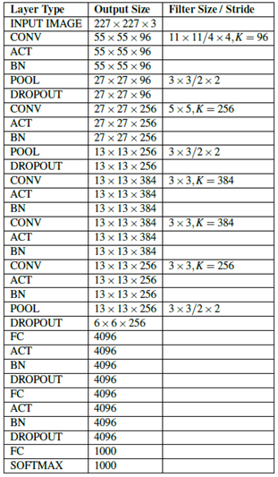 Tabular summary of the AlexNet architecture. Each layer contains the output volume size and the convolution filter size / pool size when relevant.
1. Implement AlexNet
Create mxalexnet Py file.
# import the necessary packages
import mxnet as mx

class MxAlexNet:
    @staticmethod
    def build(classes):
        # data input
        data = mx.sym.Variable("data")

        # Block #1: first CONV => RELU => POOL layer set
        conv1_1 = mx.sym.Convolution(data=data, kernel=(11, 11), stride=(4, 4), num_filter = 96)
        act1_1 = mx.sym.LeakyReLU(data=conv1_1, act_type="elu")
        bn1_1 = mx.sym.BatchNorm(data=act1_1)
        pool1 = mx.sym.Pooling(data=bn1_1, pool_type="max", kernel=(3, 3), stride=(2, 2))
        do1 = mx.sym.Dropout(data=pool1, p=0.25)

        # Use standard ReLU instead of ELU
        # # Block #1: first CONV => RELU => POOL layer set
        # conv1_1 = mx.sym.Convolution(data=data, kernel=(11, 11),stride = (4, 4), num_filter = 96)
        # bn1_1 = mx.sym.BatchNorm(data=conv1_1)
        # act1_1 = mx.sym.Activation(data=bn1_1, act_type="relu")
        # pool1 = mx.sym.Pooling(data=act1_1, pool_type="max",kernel = (3, 3), stride = (2, 2))
        # do1 = mx.sym.Dropout(data=pool1, p=0.25)

        # ReLU activation is retained, but the order of batch standardization is exchanged
        # # Block #1: first CONV => RELU => POOL layer set
        # conv1_1 = mx.sym.Convolution(data=data, kernel=(11, 11),stride = (4, 4), num_filter = 96)
        # act1_1 = mx.sym.Activation(data=conv1_1, act_type="relu")
        # bn1_1 = mx.sym.BatchNorm(data=act1_1)
        # pool1 = mx.sym.Pooling(data=bn1_1, pool_type="max",kernel = (3, 3), stride = (2, 2))
        # do1 = mx.sym.Dropout(data=pool1, p=0.25)

        # Block #2: second CONV => RELU => POOL layer set
        conv2_1 = mx.sym.Convolution(data=do1, kernel=(5, 5), pad=(2, 2), num_filter=256)
        act2_1 = mx.sym.LeakyReLU(data=conv2_1, act_type="elu")
        bn2_1 = mx.sym.BatchNorm(data=act2_1)
        pool2 = mx.sym.Pooling(data=bn2_1, pool_type="max", kernel = (3, 3), stride = (2, 2))
        do2 = mx.sym.Dropout(data=pool2, p=0.25)

        # Block #3: (CONV => RELU) * 3 => POOL
        conv3_1 = mx.sym.Convolution(data=do2, kernel=(3, 3), pad=(1, 1), num_filter=384)
        act3_1 = mx.sym.LeakyReLU(data=conv3_1, act_type="elu")
        bn3_1 = mx.sym.BatchNorm(data=act3_1)
        conv3_2 = mx.sym.Convolution(data=bn3_1, kernel=(3, 3), pad=(1, 1), num_filter=384)
        act3_2 = mx.sym.LeakyReLU(data=conv3_2, act_type="elu")
        bn3_2 = mx.sym.BatchNorm(data=act3_2)
        conv3_3 = mx.sym.Convolution(data=bn3_2, kernel=(3, 3), pad=(1, 1), num_filter=256)
        act3_3 = mx.sym.LeakyReLU(data=conv3_3, act_type="elu")
        bn3_3 = mx.sym.BatchNorm(data=act3_3)
        pool3 = mx.sym.Pooling(data=bn3_3, pool_type="max", kernel=(3, 3), stride = (2, 2))
        do3 = mx.sym.Dropout(data=pool3, p=0.25)

        # Block #4: first set of FC => RELU layers
        flatten = mx.sym.Flatten(data=do3)
        fc1 = mx.sym.FullyConnected(data=flatten, num_hidden=4096)
        act4_1 = mx.sym.LeakyReLU(data=fc1, act_type="elu")
        bn4_1 = mx.sym.BatchNorm(data=act4_1)
        do4 = mx.sym.Dropout(data=bn4_1, p=0.5)
        # Block #5: second set of FC => RELU layers
        fc2 = mx.sym.FullyConnected(data=do4, num_hidden=4096)
        act5_1 = mx.sym.LeakyReLU(data=fc2, act_type="elu")
        bn5_1 = mx.sym.BatchNorm(data=act5_1)
        do5 = mx.sym.Dropout(data=bn5_1, p=0.5)

        # softmax classifier
        fc3 = mx.sym.FullyConnected(data=do5, num_hidden=classes)
        model = mx.sym.SoftmaxOutput(data=fc3, name="softmax")
        # return the network architecture
        return model
2. Training Alex net
Create train_alexnet.py file.
# import the necessary packages
import imagenet_alexnet_config as config
from mxalexnet import MxAlexNet
import mxnet as mx
import argparse
import logging
import json
import os

# construct the argument parse and parse the arguments
ap = argparse.ArgumentParser()
ap.add_argument("-c", "--checkpoints", required=True, help="path to output checkpoint directory")
ap.add_argument("-p", "--prefix", required=True, help="name of model prefix")
ap.add_argument("-s", "--start-epoch", type=int, default=0, help="epoch to restart training at")
args = vars(ap.parse_args())

# set the logging level and output file
logging.basicConfig(level=logging.DEBUG,filename="training_{}.log".format(args["start_epoch"]),filemode="w")

# load the RGB means for the training set, then determine the batch
# size
means = json.loads(open(config.DATASET_MEAN).read())
batchSize = config.BATCH_SIZE * config.NUM_DEVICES

# construct the training image iterator
trainIter = mx.io.ImageRecordIter(
    path_imgrec=config.TRAIN_MX_REC,
    data_shape=(3, 227, 227),
    batch_size=batchSize,
    rand_crop=True,
    rand_mirror=True,
    rotate=15,
    max_shear_ratio=0.1,
    mean_r=means["R"],
    mean_g=means["G"],
    mean_b=means["B"],
    preprocess_threads=config.NUM_DEVICES * 2)

# construct the validation image iterator
valIter = mx.io.ImageRecordIter(
    path_imgrec=config.VAL_MX_REC,
    data_shape=(3, 227, 227),
    batch_size=batchSize,
    mean_r=means["R"],
    mean_g=means["G"],
    mean_b=means["B"])

# initialize the optimizer
opt = mx.optimizer.SGD(learning_rate=1e-2, momentum=0.9, wd=0.0005, rescale_grad=1.0 / batchSize)

# # initialize the optimizer
# opt = mx.optimizer.SGD(learning_rate=1e-3, momentum=0.9, wd=0.0005, rescale_grad=1.0 / batchSize)

# construct the checkpoints path, initialize the model argument and
# auxiliary parameters
checkpointsPath = os.path.sep.join([args["checkpoints"], args["prefix"]])
argParams = None
auxParams = None

# if there is no specific model starting epoch supplied, then
# initialize the network
if args["start_epoch"] <= 0:
    # build the LeNet architecture
    print("[INFO] building network...")
    model = MxAlexNet.build(config.NUM_CLASSES)
# otherwise, a specific checkpoint was supplied
else:
    # load the checkpoint from disk
    print("[INFO] loading epoch {}...".format(args["start_epoch"]))
    model = mx.model.FeedForward.load(checkpointsPath,args["start_epoch"])

    # update the model and parameters
    argParams = model.arg_params
    auxParams = model.aux_params
    model = model.symbol

# compile the model
model = mx.model.FeedForward(
    ctx=[mx.gpu(0)],
    #ctx=[mx.gpu(1), mx.gpu(2), mx.gpu(3)],
    symbol=model,
    initializer=mx.initializer.Xavier(),
    arg_params=argParams,
    aux_params=auxParams,
    optimizer=opt,
    num_epoch=90,
    begin_epoch=args["start_epoch"])

# initialize the callbacks and evaluation metrics
batchEndCBs = [mx.callback.Speedometer(batchSize, 500)]
epochEndCBs = [mx.callback.do_checkpoint(checkpointsPath)]
metrics = [mx.metric.Accuracy(), mx.metric.TopKAccuracy(top_k=5), mx.metric.CrossEntropy()]

# train the network
print("[INFO] training network...")
model.fit(
    X=trainIter,
    eval_data=valIter,
    eval_metric=metrics,
    batch_end_callback=batchEndCBs,
    epoch_end_callback=epochEndCBs)
3. Verify AlexNet
Create test_alexnet.py file.
# import the necessary packages
import imagenet_alexnet_config as config
import mxnet as mx
import argparse
import json
import os

# construct the argument parse and parse the arguments
ap = argparse.ArgumentParser()
ap.add_argument("-c", "--checkpoints", required=True, help="path to output checkpoint directory")
ap.add_argument("-p", "--prefix", required=True, help="name of model prefix")
ap.add_argument("-e", "--epoch", type=int, required=True, help="epoch # to load")
args = vars(ap.parse_args())

# load the RGB means for the training set
means = json.loads(open(config.DATASET_MEAN).read())
# construct the testing image iterator
testIter = mx.io.ImageRecordIter(
    path_imgrec=config.TEST_MX_REC,
    data_shape=(3, 227, 227),
    batch_size=config.BATCH_SIZE,
    mean_r=means["R"],
    mean_g=means["G"],
    mean_b=means["B"])

# load the checkpoint from disk
print("[INFO] loading model...")
checkpointsPath = os.path.sep.join([args["checkpoints"], args["prefix"]])
model = mx.model.FeedForward.load(checkpointsPath, args["epoch"])

# compile the model
model = mx.model.FeedForward(
    ctx=[mx.gpu(0)],
    symbol=model.symbol,
    arg_params=model.arg_params,
    aux_params=model.aux_params)

# make predictions on the testing data
print("[INFO] predicting on test data...")
metrics = [mx.metric.Accuracy(), mx.metric.TopKAccuracy(top_k=5)]
(rank1, rank5) = model.score(testIter, eval_metric=metrics)

# display the rank-1 and rank-5 accuracies
print("[INFO] rank-1: {:.2f}%".format(rank1 * 100))
print("[INFO] rank-5: {:.2f}%".format(rank5 * 100))
4. AlexNet experiment
When evaluating and comparing the performance of AlexNet, we usually use the BVLC AlexNet implementation provided by Caffe instead of the original AlexNet implementation. There are many reasons for this comparison, including different data enhancements used by Krizhevsky et al. And (now deprecated) the use of local response normalization layer (LRN). In addition, the "CaffeNet" version of AlexNet is often more accessible to the scientific community. In the rest of this section, I will compare my results with the CaffeNet benchmark, but still refer to the original paper by Krizhevsky et al.
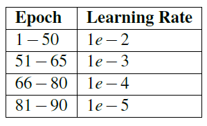 Table 6.2: learning rate plan used for experimental #1 training of AlexNet on ImageNet.
4.1 Experiment 1
In the first AlexNet experiment, I decided to prove empirically why we placed batch standardization layers after activation rather than before activation. I also used standard ReLU instead of ELU to obtain the baseline of model performance (Krizhevsky et al. Used ReLU in their experiments). Therefore, I modified the mxalexnet.py file detailed earlier in this chapter to reflect batch normalization and activation changes, as shown below:
# Block #1: first CONV => RELU => POOL layer set
conv1_1 = mx.sym.Convolution(data=data, kernel=(11, 11),stride = (4, 4), num_filter = 96)
bn1_1 = mx.sym.BatchNorm(data=conv1_1)
act1_1 = mx.sym.Activation(data=bn1_1, act_type="relu")
pool1 = mx.sym.Pooling(data=act1_1, pool_type="max",kernel = (3, 3), stride = (2, 2))
do1 = mx.sym.Dropout(data=pool1, p=0.25)
Using SGD to train AlexNet, the initial learning rate is 1e-2, the momentum term is 0.9, and the L2 weight attenuation is 0.0005.
Progress is monitored approximately every 10 epochs. One of the most serious mistakes I see new deep learning practitioners make is checking their training charts too often. In most cases, you need 10-15 epoch contexts to make decisions about whether the network is indeed over fitting, under fitting, etc. After 70 epochs, I plotted my training loss and accuracy (Figure 6.1, top EFT). At this time, the accuracy of verification and training basically stagnated at about 49-50%, which clearly shows that the learning rate can be reduced to further improve the accuracy.
So I edit train_ alexnet. Line 53 and 54 of Py update my learning rate to 1e-3:
# initialize the optimizer
opt = mx.optimizer.SGD(learning_rate=1e-3, momentum=0.9, wd=0.0005, rescale_grad=1.0 / batchSize)
Note how the learning rate decreases from 1e-2 to 1e-3, but all other SGD parameters remain unchanged. Then I restart training from epoch 50 using the following command:
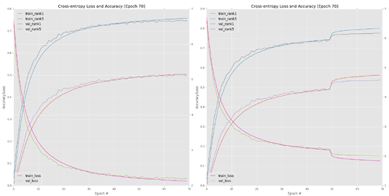
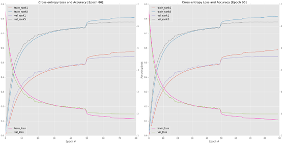 Figure 6.1: upper left corner: let AlexNet train to the 70th period, and the learning rate is 1e-2. Note how the accuracy of level 1 stagnates at about 49%. I stopped training after epoch70 and decided to restart training at epoch50. Top right: restart training from epoch50, and the learning rate is 1e-3. An order of magnitude decrease in a allows the network to "jump" to higher accuracy / lower loss. Lower left corner: restart training from epoch65, a=1e-4. Bottom right: 80-90 epoch at a=1e-5.
Monitor the progress of AlexNet, Until 70epoch (Figure 6.1, top right). The first key conclusion you should check from this figure is how reducing my learning rate from 1e-2 to 1e-3 leads to a sharp increase in accuracy and a sharp decrease in loss after the 50th period - this increase in accuracy and loss is normal when you train deep neural networks on large data sets. By reducing learning For the learning rate, we allow our network to drop to lower loss areas, because the previous learning rate is too large for the optimizer to find these areas. Remember, the goal of training deep learning network is not necessarily to find global minimum or even local minimum; Instead of simply finding an area where the loss is low enough.
However, at a later stage, I began to notice the stagnation of verification loss / accuracy (although training accuracy / loss continued to improve). This stagnation is often an obvious sign that overfitting began to occur, but the gap between verification and training loss is acceptable, so I am not too worried. I updated my learning rate to 1e-4 (also, by editing lines 53 and 54 of train_alexnet.py) and restart the training from epoch 65:

The verification loss / accuracy improved slightly, but at this time the learning rate began to become too small - in addition, we began to over fit the training data (Figure 6.1, lower left corner).
Finally, my network is allowed to train more than 10 epochs (80-90) with 1e-5 learning rate:

Figure 6.1 (bottom right) contains the result chart of the last ten periods. Further training after phase 90 is unnecessary because the verification loss / accuracy has stopped improving, while the training loss continues to decline, which puts us at risk of over fitting. At the end of epoch 90, I obtained 54.14% rank-1 accuracy and 77.90% rank-5 accuracy on the verification data. Yes For the first experiment, this accuracy is very reasonable, but it does not fully meet my expectations for AlexNet level performance. The BVLC CaffeNet reference model reports that the performance is about 57% rank-1 accuracy and 80% rank-5 accuracy.
4.2} Experiment 2
The purpose of this experiment is to build on the previous experiment and show why we place batch normalization layers after activation. I retained ReLU activation, but exchanged the order of batch standardization, as shown in the following code block:
#ReLU activation is retained, but the order of batch standardization is exchanged
# Block #1: first CONV => RELU => POOL layer set
conv1_1 = mx.sym.Convolution(data=data, kernel=(11, 11),stride = (4, 4), num_filter = 96)
act1_1 = mx.sym.Activation(data=conv1_1, act_type="relu")
bn1_1 = mx.sym.BatchNorm(data=act1_1)
pool1 = mx.sym.Pooling(data=bn1_1, pool_type="max",kernel = (3, 3), stride = (2, 2))
do1 = mx.sym.Dropout(data=pool1, p=0.25)
Similarly, I used the same optimizer parameters as SGD. The initial learning rate was 1e-2, the momentum was 0.9, and the L2 weight attenuation was 0.0005. Table 6.3 includes my time and related learning rate plans. I started training AlexNet with the following command:

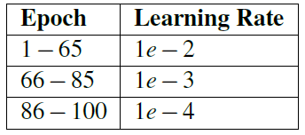
Table 6.3: learning rate plan used in experimental #2 and experimental #3 training of AlexNet on ImageNet.
Around epoch 65, I noticed that the verification loss and accuracy stagnated (Figure 6.2, upper left corner). Therefore, I stopped training, adjusted my learning rate to 1e-3, and then restarted training from the 65th Epoch:

Similarly, when the verification accuracy / loss is stable, We can see the characteristic jump of accuracy by reducing the learning rate (Figure 6.2, upper right corner). In the 85th period, I reduced my learning rate again, this time from 1e-3 to 1e-4, and allowed the network to train for another 15 periods, and then verified that the loss / accuracy stopped improving (Figure 6.2, bottom).
Check the experiment log and note that the accuracy of rank-1 and rank-5 is 56.72% and 79.62%, which is much better than my previous experiment of placing batch normalization layer before activation. In addition, these results are completely within the statistical range of real AlexNet level performance.
4.3} Experiment 3
Since my previous experiments showed that placing batch standardization after activation would produce better results, I decided to replace standard ReLU activation with ELU activation. In my experience, replacing ReLU with ELU can usually improve your classification accuracy on ImageNet dataset by 1-2%. Therefore, my conv = > ReLU block now becomes:
# Block #1: first CONV => RELU => POOL layer set
conv1_1 = mx.sym.Convolution(data=data, kernel=(11, 11), stride=(4, 4), num_filter = 96)
act1_1 = mx.sym.LeakyReLU(data=conv1_1, act_type="elu")
bn1_1 = mx.sym.BatchNorm(data=act1_1)
pool1 = mx.sym.Pooling(data=bn1_1, pool_type="max", kernel=(3, 3), stride=(2, 2))
do1 = mx.sym.Dropout(data=pool1, p=0.25)
Notice how to place the batch normalization layer after activation and how to replace the ELU with ReLU. In this experiment, I used the same SGD optimizer parameters as the previous two experiments. I also followed the same learning rate plan in the second experiment (table 6.3).
To copy my experiment, you can use the following command:

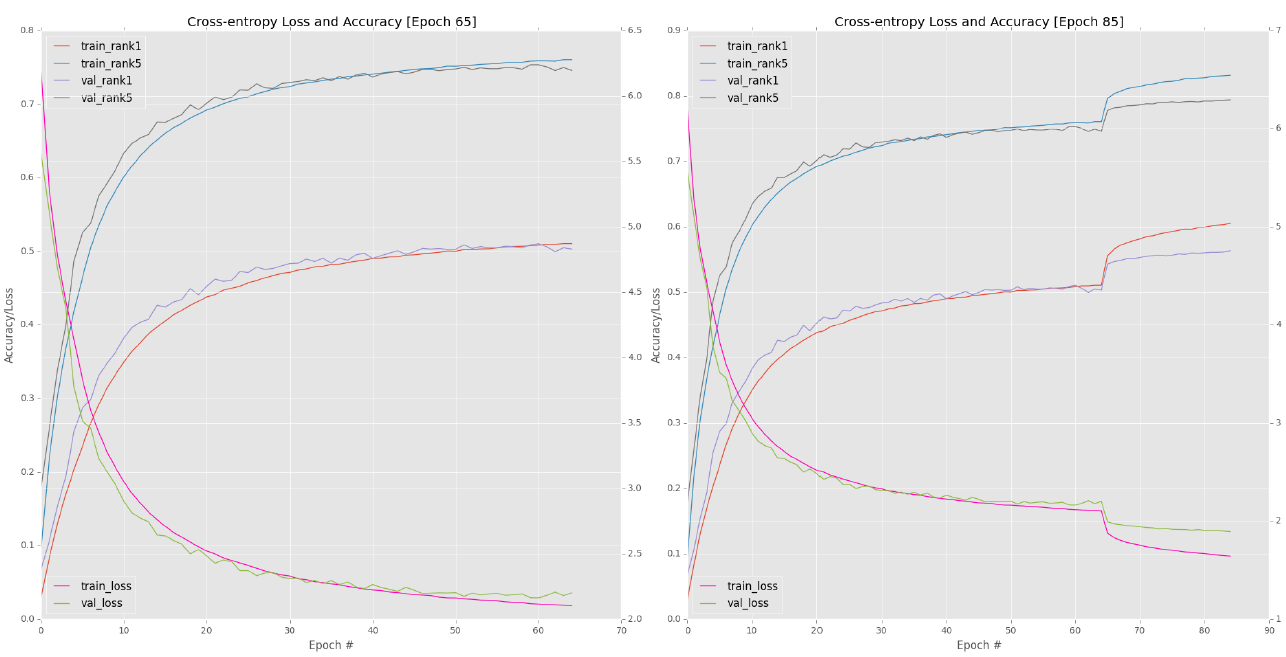
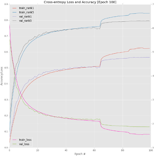 Figure 6.2: top right: when placing activation before batch normalization, the learning rate of the first 65 epoch s is 1e-2. Upper left: reducing a to 1e-3 leads to a sharp increase in accuracy and a reduction in loss; However, the decline rate of training loss is significantly faster than that of verification loss. Bottom: for the 85th-100th period, a finally drops to 1e-4.

The first command starts training from the first epoch, and the initial learning rate is 1e-2. The second command restarts training at the 65th epoch, with a learning rate of 1e-3. The last command resumed training in the 85th period, with a learning rate of 1e-4.
A complete graph of training and verification loss / accuracy can be seen in Figure 6.3. Similarly, you can see that the learning rate is adjusted by an order of magnitude during rounds 65 and 85, and the jump becomes less obvious as the learning rate decreases. I don't want to train the past 100 eras because Alex net obviously began to over fit the training data, and the verification accuracy / loss is still stagnant. The larger the gap, the more serious the over fitting is. Therefore, we apply the "early stop" regularization standard to prevent further over fitting.
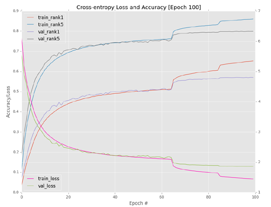 Figure 6.3: in our final AlexNet + ImageNet experiment, we replaced ReLU with ELU, and obtained 57.00% / 75.52% validation rank-1/rank-5 accuracy and 59.80% test rank-1/rank-5 accuracy% / 81.75%.
Checking the accuracy of the 100th period, I found that I obtained 57.00% rank-1 accuracy and 79.52% rank-5 accuracy on the validation data set. This result is only a little better than my second experiment, but it's very interesting when I use test_ alexnet. What happens when a py script evaluates on a test set:

I summarize the results in table 6.4. As you can see here, I have achieved 59.80% rank-1 and 81.75% rank-5 accuracy on the test set, which is certainly higher than the AlexNet accuracy reported in most independent papers and publications. For your convenience, I included the weight of this AlexNet experiment in the ImageNet Bundle you downloaded.
In general, the purpose of this section is to give you an understanding of the types of experiments required to obtain a reasonably performing model on an ImageNet dataset. In fact, my lab log contains 25 independent Alex Net + ImageNet experiments, too many to be included in this book. Instead, I chose the ones that best represent the important changes I have made to the network architecture and optimizer. Remember that for most deep learning problems, you will run 10-100 experiments (or even more in some cases) before you get a model that performs well on validation and test data.
 Table 6.4: evaluating AlexNet on the ImageNet test set. Our results are better than the standard Caffe reference model used to benchmark Alex net
Unlike other programming fields, you can write a function and run it forever. On the contrary, there are many areas that need to be fine tuned. After adjusting the parameters, you will get a CNN reward for good performance, but before that, please wait patiently and record your results! It's valuable to write down what works and what doesn't -- notes that will allow you to reflect on your experiments and identify new ways to pursue them.
5. Summary
In this chapter, we implement the AlexNet architecture using the mxnet library, and then train it on the ImageNet dataset. This chapter is long because we need a comprehensive view of the AlexNet architecture, training scripts and evaluation scripts. Now that we have defined our training and evaluation Python scripts, we will be able to reuse them in future experiments to make training and evaluation easier - our main task is to implement the actual network architecture.
Our experiments enabled us to identify two important points:
1. In most cases, batch normalization after activation (rather than before) will lead to higher classification accuracy / lower loss.
2. Replacing ReLU with ELU can give you a small improvement in classification accuracy.
Overall, we can obtain 59.80% rank-1 and 81.75% rank-5 accuracy on ImageNet, which is better than the standard Caffe reference model used to benchmark AlexNet.