Programmer's view of love: love is a dead cycle, once executed, it will fall into; Falling in love with someone is a memory leak - you can never release it; When you really love someone, that is constant limit, which will never change; Girlfriend is a private variable, which can only be called by my class; Lover is a pointer. You must pay attention when using it, or it will bring great disaster.

Neural network is the basis of deep learning. I understand that neural network is the structure that can fit any kind of generalized linear model. BP algorithm is the algorithm for solving parameter w. the basis of neural network and weight learning algorithm are BP learning algorithm. The signal "forward propagation (FP)" calculates the loss and "back propagation (BP)" returns the error; Modify the weight of each layer according to the error value and continue the iteration.

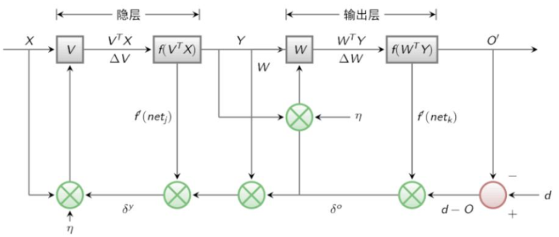
Output layer error
O represents the predicted result and d represents the real result; The coefficient is calculated for the convenience of derivation

Like general neural networks, BP neural networks conduct FP conduction first, that is, forward conduction. In the case, only one hidden layer is set, so there are two parameter layers: W1, B1; w2,b2; Row and column of W parameter matrix: the number of neurons in the behavior output layer, and column is the number of neurons in the input layer.
The result of the hidden layer: O1=sigmoid(a1)=sigmoid(w1.x.T+b1). The hidden layer uses the sigmoid activation function
Output result: O2=a2=W2*O1+b2, the last layer does not use the activation function
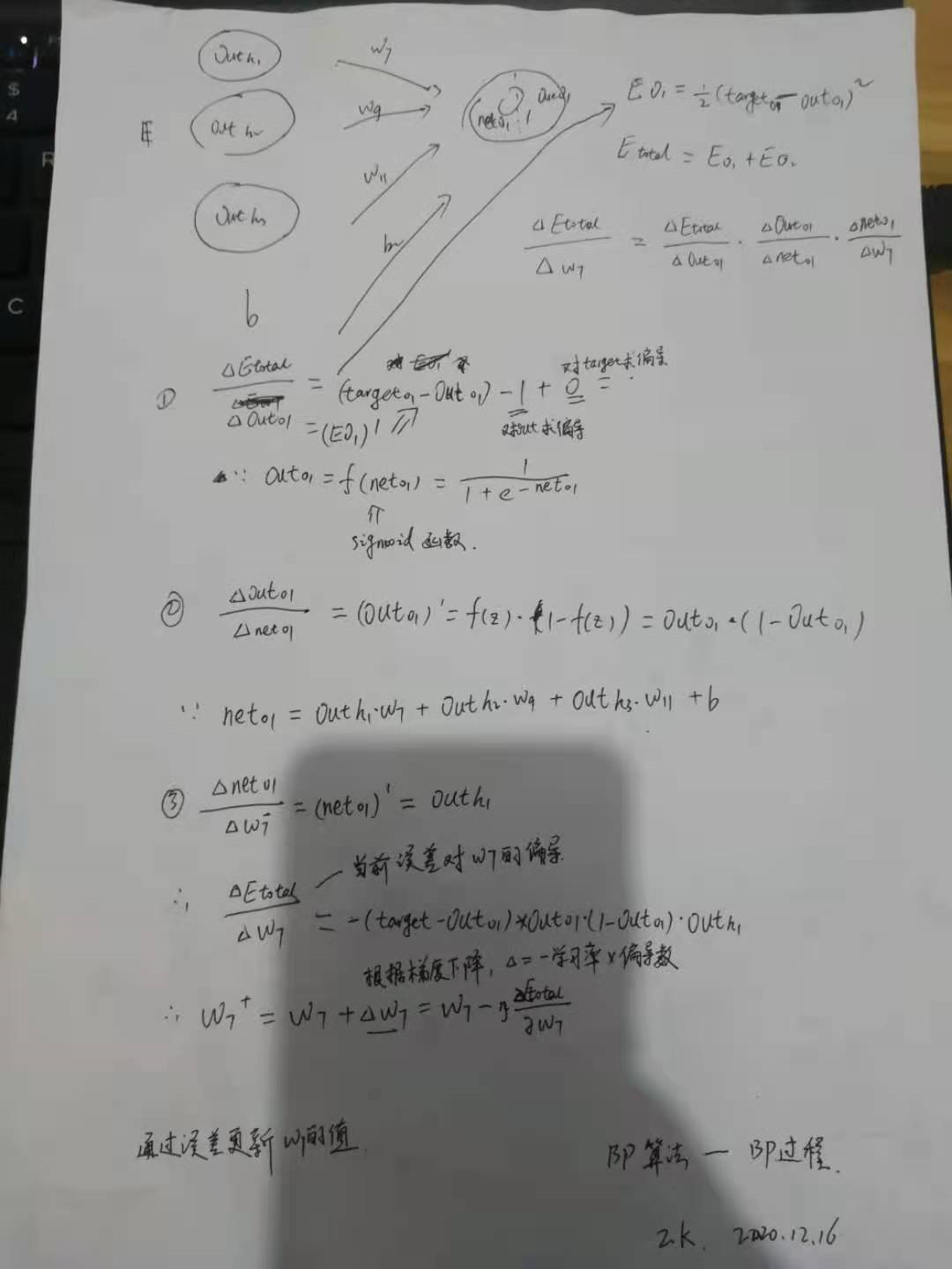
The loss function cost=1/2(O2-y)^2. In the brackets is the square of the predicted value minus the actual value, while the error term we often use err=y-O2. In fact, err can also be equal to O2-y, so the err form determines whether we need to add a negative sign to the following err. Because the partial derivative of cost to O2 is (O2-y), the conversion of the relationship between err and (O2-y) needs special attention.
Here we define err=y-O2;
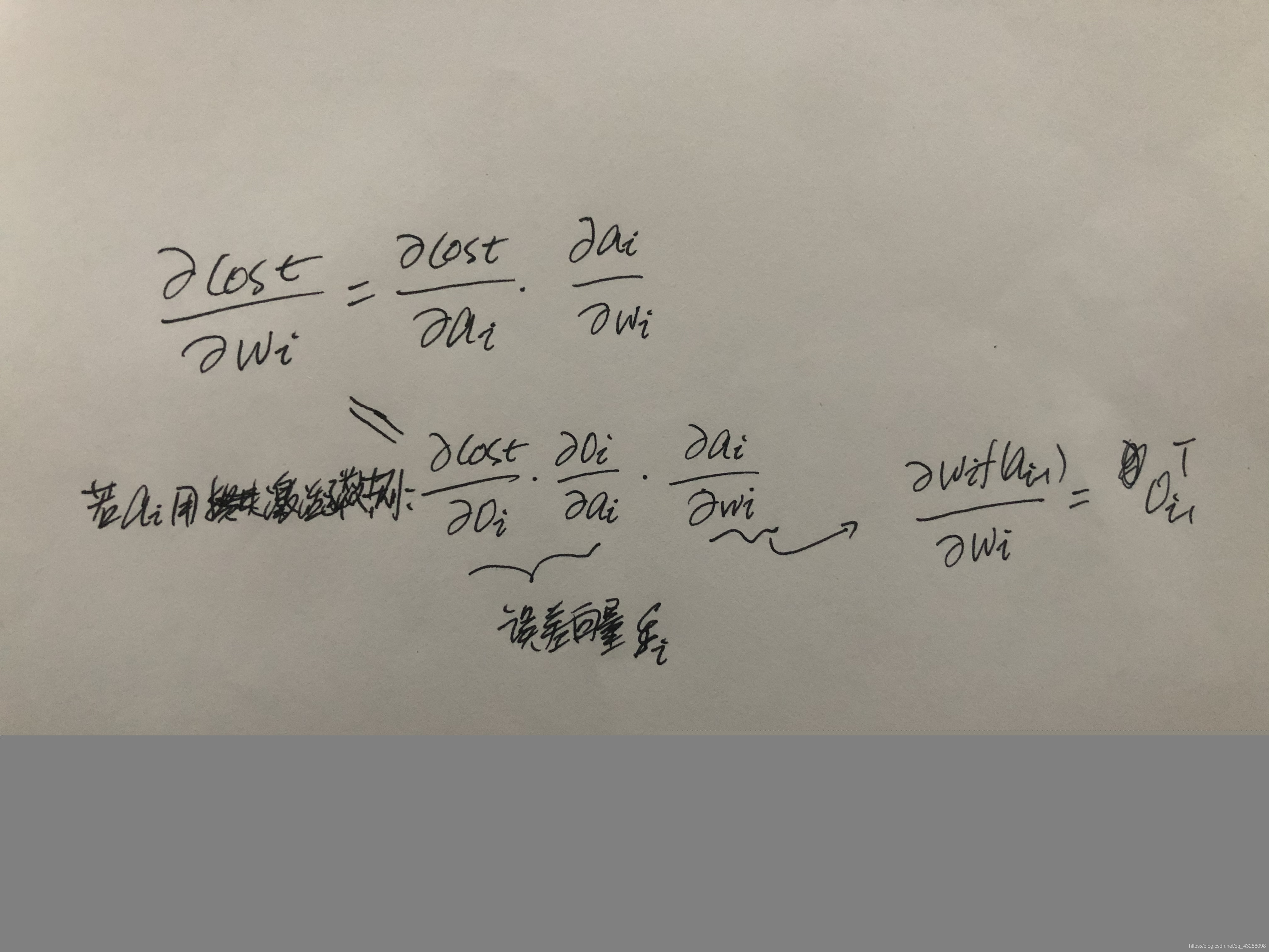
The loss function obtains the partial derivative of Wi, that is, the gradient value. The derivative process uses the differential chain derivative
As shown in the figure below, the gradient is equal to the error term multiplied by the input value of the previous layer. For the Wi of the last layer, we can get equal to - (y-oi) oi-1 T. That is - erroi-1 T. In the last layer, we did not convert the activation function of a2, so there was no derivation of the activation function about a2, that is, the derivation of O2 from a2 was 1, so it was ignored

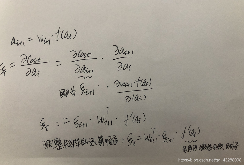
The loss function biases ai to obtain the error vector. The derivative process uses differential chain derivation:

import numpy as np
import  pandas as pd
import matplotlib as mpl
import  matplotlib.pyplot as  plt
from sklearn.preprocessing import  MinMaxScaler

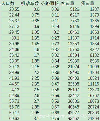
df=pd.read_csv('traffic_data.csv',encoding='GBK')
print(df.head)

x=df[['Population','Number of motor vehicles','Highway area']]
y=df[['Passenger volume','the volume of freight transport']]

print(x)
print(y)

#Normalize the maximum and minimum values of the data
x_scaler=MinMaxScaler(feature_range=(-1,1))
y_scaler=MinMaxScaler(feature_range=(-1,1))

x=x_scaler.fit_transform(x)
y=y_scaler.fit_transform(y)

#Transpose the sample and perform matrix operation
sample_in=x.T
sample_out=y.T

#BP neural network parameters
max_epochs=60000 #Number of loop iterations
learn_rate=0.035  #Learning rate
mse_final=6.5e-4  #Set a threshold of mean square error, and if it is less than it, the iteration will be stopped
sample_number=x.shape[0]  #Number of samples
input_number=x.shape[1]  #Input feature number
output_number=y.shape[1]  #Number of output targets
hidden_units=8 #Number of hidden layer neurons
print(sample_number,input_number,output_number)


#Define activation function Sigmod
# import math
def sigmoid(z):
    return  1/(1+np.exp(-z))

def sigmoid_delta(z): #partial derivative
    return 1/((1+np.exp(-z))**2)*np.exp(-z)

print(sigmoid(0),sigmoid_delta(0))

#A hidden layer
#W1 matrix: M rows and N columns, M is equal to the number of neurons in this layer, and N is equal to the number of input features
W1=0.5*np.random.rand(hidden_units,input_number)-0.1
b1=0.5*np.random.rand(hidden_units,1)-0.1

W2=0.5*np.random.rand(output_number,hidden_units)-0.1
b2=0.5*np.random.rand(output_number,1)-0.1

mse_history=[]  #Empty list to store iteration errors
#Do not set activation function
for i in range(max_epochs):
    #FP
    hidden_out=sigmoid(np.dot(W1,sample_in)+b1)  #np.dot moment matrix multiplication, hidden_ The out1 result is 8 rows and 20 columns
    network_out=np.dot(W2,hidden_out)+b2  #np.dot matrix multiplication, W2 is 2 rows and 8 columns, then the output result is 2 rows and 20 columns
    #error
    err=sample_out-network_out
    mse_err=np.average(np.square(err)) #Mean square error
    mse_history.append(mse_err)
    if mse_err<mse_final:
        break
    #BP
    #Error vector
    delta2=-err #Error of the last layer
    delta1=np.dot(W2.transpose(),delta2)*sigmoid_delta(hidden_out)  #The error vector of the previous layer. This layer is hidden_out uses sigmoid to activate the function. It is necessary to activate hidden_ Find the partial derivative; Note that the last step is the dot multiplication of two matrices, which are two matrices with exactly the same dimension
    #Gradient: partial derivative of loss function
    delta_W2=np.dot(delta2,hidden_out.transpose())
    delta_W1=np.dot(delta1,sample_in.transpose())
    delta_b2=np.dot(delta2,np.ones((sample_number,1)))
    delta_b1=np.dot(delta1,np.ones((sample_number,1)))
    W2-=learn_rate*delta_W2
    b2-=learn_rate*delta_b2
    W1-=learn_rate*delta_W1
    b1-=learn_rate*delta_b1


#Loss value drawing
print(mse_history)
loss=np.log10(mse_history)
min_mse=min(loss)
plt.plot(loss,label='loss')
plt.plot([0,len(loss)],[min_mse,min_mse],label='min_mse')
plt.xlabel('iteration')
plt.ylabel('MSE loss')
plt.title('Log10 MSE History',fontdict={'fontsize':18,'color':'red'})
plt.legend()
plt.show()


#Comparison between model predicted output and actual output
hidden_out=sigmoid(np.dot(W1,sample_in)+b1)
network_out=np.dot(W2,hidden_out)+b2

#Invert to get actual value:
network_out=y_scaler.inverse_transform(network_out.T)
sample_out=y_scaler.inverse_transform(y)

#Solve the problem that Chinese pictures cannot be displayed
plt.rcParams['font.sans-serif'] = [u'SimHei']
plt.rcParams['axes.unicode_minus'] = False

plt.figure(figsize=(8, 6))
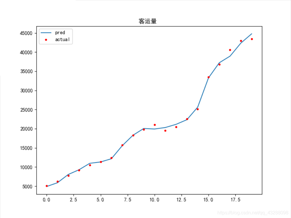
plt.plot(network_out[:,0],label='pred')
plt.plot(sample_out[:,0],'r.',label='actual')
plt.title('Passenger volume ',)
plt.legend()
plt.show()



plt.figure(figsize=(8, 6))
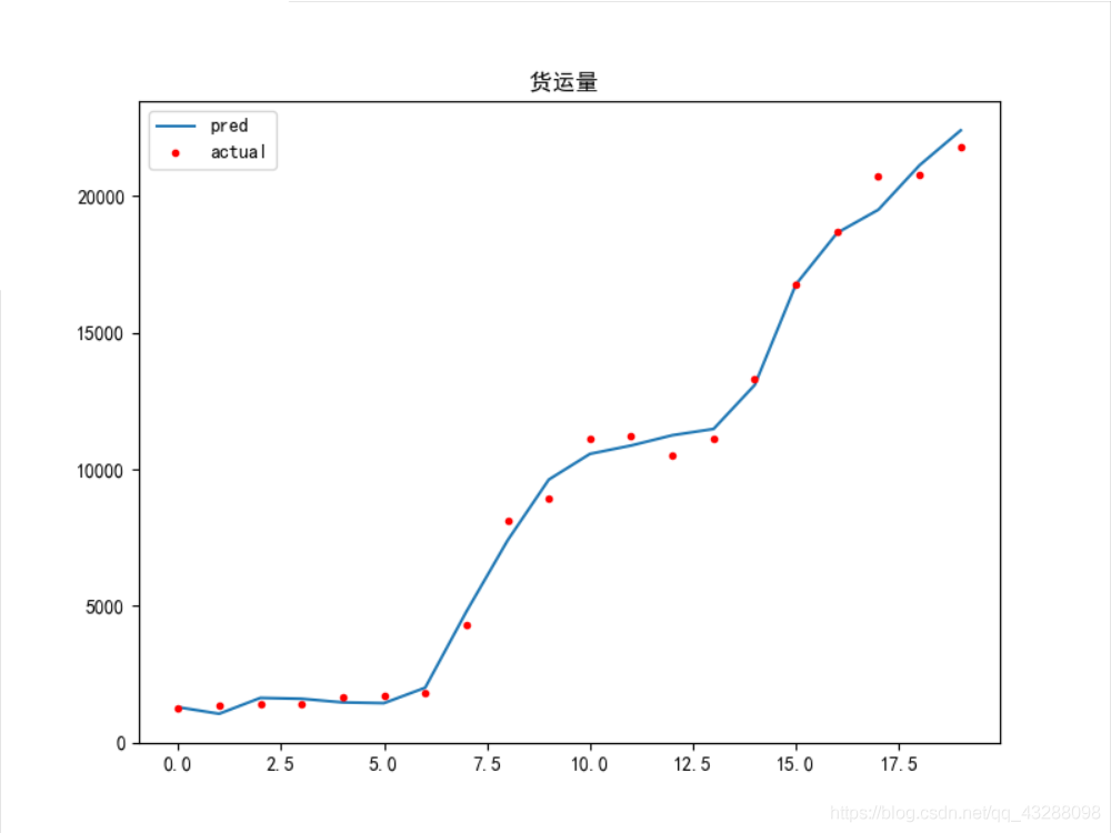
plt.plot(network_out[:,1],label='pred')
plt.plot(sample_out[:,1],'r.',label='actual')
plt.title('the volume of freight transport ')
plt.legend()
plt.show()

The simulation results are shown as follows:
This is the result of an iteration:

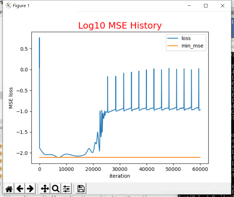
It can be seen that the fitting result is not very good, and the predicted value deviates greatly from the actual value
The better model results are given below

traffic_ data. The CSV data is as follows

Question:
1. It can be seen from here that it is very important to set the initial value of parameters. The solution may be to train several times to get a better model result
Information:
Neural network, understanding and derivation of BP algorithm https://zhuanlan.zhihu.com/p/45190898
BP algorithm of neural network_ Actual combat prediction case https://www.bilibili.com/video/BV1a7411J7SR?t=2522