Chapter 6 of Volume III trains GoogLeNet on ImageNet

GoogLeNet and VGGNet were the leaders in the 2014 ImageNet large-scale visual recognition challenge (ILSVRC). GoogLeNet slightly surpassed VGGNet and ranked first. GoogLeNet also has the additional advantage of being significantly smaller than VGG16 and VGG19. The model size is only 28.12MB, while VGG exceeds 500MB.

However, many researchers (including authors) have encountered difficulties in independent ImageNet experimental results. For example, the ranking maintained by vlfeat (an open source library for computer vision and machine learning) reports that VGG16 and VGG19 perform significantly better than GoogLeNet [24]. It is unclear why this is so.

1. Learn about GoogLeNet

1.1 Inception module

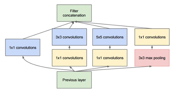The original inception module used in GoogLeNet. The first mock exam is Inception module, which calculates the convolution of 1*1, 3* 3 and 5*5 in the same module of the network to act as "multi-level feature extractor".

The concept module is a four branch microarchitecture used in the GoogLeNet architecture (Figure). The main purpose of the concept module is to learn multi-scale features (1 * 1, 3 * 3 and 5 * 5 filters), and then let the network "decide" which weights are most important according to the optimization algorithm.

1.2 GoogLeNet architecture

We will implement as close to the original GoogLeNet as possible.

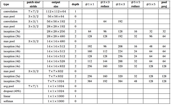Complete GoogLeNet architecture.

We started with a 7 * 7 convolution with a step size of 2 * 2, and we learned a total of 64 filters. The maximum POOL operation is called immediately. The kernel size is 3 * 3 and the step size is 2 * 2. These CONV and POOL layers reduce our input volume size from 224 * 224 * 3 to 56 * 56 * 64 (note how much the spatial size of the image decreases).

From there, apply another CONV layer, where we learn 192 3 filters. Then there is the POOL layer, which reduces our spatial dimension to 28 192. Next, we stack two Inception modules (named 3a and 3b), followed by another POOL.

In order to learn more in-depth and rich functions, we stacked five Inception modules (4a-4e), followed by a POOL. Two other Inception modules are applied (5a and 5b), so that our output volume size is 7 7 1024. In order to avoid using the full connection layer, we can use global average pooling to reduce the average of 7 * 7 volumes to 1 * 1 * 1024. Then we can apply dropout to reduce over fitting. Segdi et al. Suggest using a 40% dropout rate; however, 50% is often the standard for most networks - in this case , we will follow the original implementation as much as possible and use 40%. After dropout, we apply a unique full connection layer in the whole architecture, where the number of nodes is the total number of class labels (1000), followed by a softmax classifier.

1.3 implementation of GoogLeNet

We now implement GoogLeNet using Python and mxnet libraries. Create a file called mxgooglenet Py.

# import the necessary packages
import mxnet as mx

class MxGoogLeNet:
    @staticmethod
    def conv_module(data, K, kX, kY, pad=(0, 0), stride=(1, 1)):
        # define the CONV => BN => RELU pattern
        conv = mx.sym.Convolution(data=data, kernel=(kX, kY), num_filter=K, pad=pad, stride=stride)
        bn = mx.sym.BatchNorm(data=conv)
        act = mx.sym.Activation(data=bn, act_type="relu")

        # return the block
        return act

    @ staticmethod
    def inception_module(data, num1x1, num3x3Reduce, num3x3, num5x5Reduce, num5x5, num1x1Proj):
        # the first branch of the Inception module consists of 1x1
        # convolutions
        conv_1x1 = MxGoogLeNet.conv_module(data, num1x1, 1, 1)

        # the second branch of the Inception module is a set of 1x1
        # convolutions followed by 3x3 convolutions
        conv_r3x3 = MxGoogLeNet.conv_module(data, num3x3Reduce, 1, 1)
        conv_3x3 = MxGoogLeNet.conv_module(conv_r3x3, num3x3, 3, 3, pad=(1, 1))

        # the third branch of the Inception module is a set of 1x1
        # convolutions followed by 5x5 convolutions
        conv_r5x5 = MxGoogLeNet.conv_module(data, num5x5Reduce, 1, 1)
        conv_5x5 = MxGoogLeNet.conv_module(conv_r5x5, num5x5, 5, 5, pad = (2, 2))

        # the final branch of the Inception module is the POOL +
        # projection layer set
        pool = mx.sym.Pooling(data=data, pool_type="max", pad=(1, 1), kernel = (3, 3), stride = (1, 1))
        conv_proj = MxGoogLeNet.conv_module(pool, num1x1Proj, 1, 1)

        # concatenate the filters across the channel dimension
        concat = mx.sym.Concat(*[conv_1x1, conv_3x3, conv_5x5, conv_proj])
        # return the block
        return concat

    @staticmethod
    def build(classes):
        # data input
        data = mx.sym.Variable("data")

        # Block #1: CONV => POOL => CONV => CONV => POOL
        conv1_1 = MxGoogLeNet.conv_module(data, 64, 7, 7, pad=(3, 3), stride=(2, 2))
        pool1 = mx.sym.Pooling(data=conv1_1, pool_type="max", pad=(1, 1), kernel=(3, 3), stride=(2, 2))
        conv1_2 = MxGoogLeNet.conv_module(pool1, 64, 1, 1)
        conv1_3 = MxGoogLeNet.conv_module(conv1_2, 192, 3, 3, pad=(1, 1))
        pool2 = mx.sym.Pooling(data=conv1_3, pool_type="max", pad=(1, 1), kernel=(3, 3), stride=(2, 2))

        # Block #3: (INCEP * 2) => POOL
        in3a = MxGoogLeNet.inception_module(pool2, 64, 96, 128, 16, 32, 32)
        in3b = MxGoogLeNet.inception_module(in3a, 128, 128, 192, 32, 96, 64)
        pool3 = mx.sym.Pooling(data=in3b, pool_type="max", pad=(1, 1), kernel=(3, 3), stride=(2, 2))

        # Block #4: (INCEP * 5) => POOL
        in4a = MxGoogLeNet.inception_module(pool3, 192, 96, 208, 16,48, 64)
        in4b = MxGoogLeNet.inception_module(in4a, 160, 112, 224, 24,64, 64)
        in4c = MxGoogLeNet.inception_module(in4b, 128, 128, 256, 24,64, 64)
        in4d = MxGoogLeNet.inception_module(in4c, 112, 144, 288, 32,64, 64)
        in4e = MxGoogLeNet.inception_module(in4d, 256, 160, 320, 32,128, 128)
        pool4 = mx.sym.Pooling(data=in4e, pool_type="max", pad=(1, 1), kernel=(3, 3), stride=(2, 2))

        # Block #5: (INCEP * 2) => POOL => DROPOUT
        in5a = MxGoogLeNet.inception_module(pool4, 256, 160, 320, 32, 128, 128)
        in5b = MxGoogLeNet.inception_module(in5a, 384, 192, 384, 48, 128, 128)
        pool5 = mx.sym.Pooling(data=in5b, pool_type="avg", kernel=(7, 7), stride=(1, 1))
        do = mx.sym.Dropout(data=pool5, p=0.4)

        # softmax classifier
        flatten = mx.sym.Flatten(data=do)
        fc1 = mx.sym.FullyConnected(data=flatten, num_hidden=classes)
        model = mx.sym.SoftmaxOutput(data=fc1, name="softmax")
        # return the network architecture
        return model

1.4 training GoogLeNet

1. Create imagenet_googlenet_config.py file. Refer to the link below,
Reading notes Deep Learning for Computer Vision with Python - Volume 3, Chapter 3, preparing ImageNet (2) _bashendixie5's blog - CSDN blog Volume 3, Chapter 3, preparing ImageNet (2) 1. Building ImageNet datasets the overall goal of building ImageNet datasets is to enable us to train convolutional neural networks from scratch. Therefore, we will review building ImageNet datasets in the context of preparing for CNN. To do this, we will first define a configuration file that stores all relevant image paths, plain text paths and what we want Any other settings included. We'll define a python class called ImageNetHelper that allows us to build quickly and easilyhttps://blog.csdn.net/bashendixie5/article/details/122149332 Only modify the following

BATCH_SIZE = 128

NUM_DEVICES = 3

Using three GPU s, I can complete one epoch every 1.7 hours or 14 epochs a day.

2. Create a train_googlenet.py file.

# import the necessary packages
import imagenet_googlenet_config as config
from mxgooglenet import MxGoogLeNet
import mxnet as mx
import argparse
import logging
import json
import os

# construct the argument parse and parse the arguments
ap = argparse.ArgumentParser()
ap.add_argument("-c", "--checkpoints", required=True, help="path to output checkpoint directory")
ap.add_argument("-p", "--prefix", required=True, help="name of model prefix")
ap.add_argument("-s", "--start-epoch", type=int, default=0, help="epoch to restart training at")
args = vars(ap.parse_args())

# set the logging level and output file
logging.basicConfig(level=logging.DEBUG, filename="training_{}.log".format(args["start_epoch"]), filemode="w")

# load the RGB means for the training set, then determine the batch
# size
means = json.loads(open(config.DATASET_MEAN).read())
batchSize = config.BATCH_SIZE * config.NUM_DEVICES

# construct the training image iterator
trainIter = mx.io.ImageRecordIter(
    path_imgrec=config.TRAIN_MX_REC,
    data_shape=(3, 224, 224),
    batch_size=batchSize,
    rand_crop=True,
    rand_mirror=True,
    rotate=15,
    max_shear_ratio=0.1,
    mean_r=means["R"],
    mean_g=means["G"],
    mean_b=means["B"],
    preprocess_threads=config.NUM_DEVICES * 2)

# construct the validation image iterator
valIter = mx.io.ImageRecordIter(
    path_imgrec=config.VAL_MX_REC,
    data_shape=(3, 224, 224),
    batch_size=batchSize,
    mean_r=means["R"],
    mean_g=means["G"],
    mean_b=means["B"])

# initialize the optimizer
opt = mx.optimizer.Adam(learning_rate=1e-3, wd=0.0002, rescale_grad=1.0 / batchSize)

# construct the checkpoints path, initialize the model argument and
# auxiliary parameters
checkpointsPath = os.path.sep.join([args["checkpoints"], args["prefix"]])
argParams = None
auxParams = None

#if there is no specific model starting epoch supplied, then
# initialize the network
if args["start_epoch"] <= 0:
    # build the LeNet architecture
    print("[INFO] building network...")
    model = MxGoogLeNet.build(config.NUM_CLASSES)

    # otherwise, a specific checkpoint was supplied
else:
    # load the checkpoint from disk
    print("[INFO] loading epoch {}...".format(args["start_epoch"]))
    model = mx.model.FeedForward.load(checkpointsPath,
    args["start_epoch"])

    # update the model and parameters
    argParams = model.arg_params
    auxParams = model.aux_params
    model = model.symbol

# compile the model
model = mx.model.FeedForward(
    ctx=[mx.gpu(0), mx.gpu(1), mx.gpu(2)],
    symbol=model,
    initializer=mx.initializer.Xavier(),
    arg_params=argParams,
    aux_params=auxParams,
    optimizer=opt,
    num_epoch=90,
    begin_epoch=args["start_epoch"])

# initialize the callbacks and evaluation metrics
batchEndCBs = [mx.callback.Speedometer(batchSize, 250)]
epochEndCBs = [mx.callback.do_checkpoint(checkpointsPath)]
metrics = [mx.metric.Accuracy(), mx.metric.TopKAccuracy(top_k=5), mx.metric.CrossEntropy()]

# train the network
print("[INFO] training network...")
model.fit(
    X=trainIter,
    eval_data=valIter,
    eval_metric=metrics,
    batch_end_callback=batchEndCBs,
    epoch_end_callback=epochEndCBs)

2. Evaluate GoogLeNet

Use the test in the previous chapter_ alexnet. py . There are no changes to the script because test_ *. In this chapter The PY script is designed to be a template that can be applied and re applied to any CNN trained on ImageNet.

3. GoogLeNet experiment

The results of ILSVRC 2014 show that GoogLeNet slightly beat vggnet in #1 the position [26]; However, many deep learning researchers (including myself) find it difficult to reproduce these exact results [24] - the results should be at least equivalent to VGG. The paper of Szegedy et al may lack the parameter settings that I and others lack in the training process.

In any case, it is still interesting to review the experiment and thinking process used by GoogLeNet and achieve reasonable accuracy (i.e. better than AlexNet, but not as good as VGG).

3.1 GoogLeNet experiment #1

In the first GoogLeNet experiment, the SGD optimizer is used, and the initial learning rate is 1e-2, which is the basic learning rate recommended by the author, as well as the momentum term 0.9 and L2 weight attenuation 0.0002. As far as I know, these optimizer parameters are exact parameters of Szegedy et al. Then I started training with the following commands:

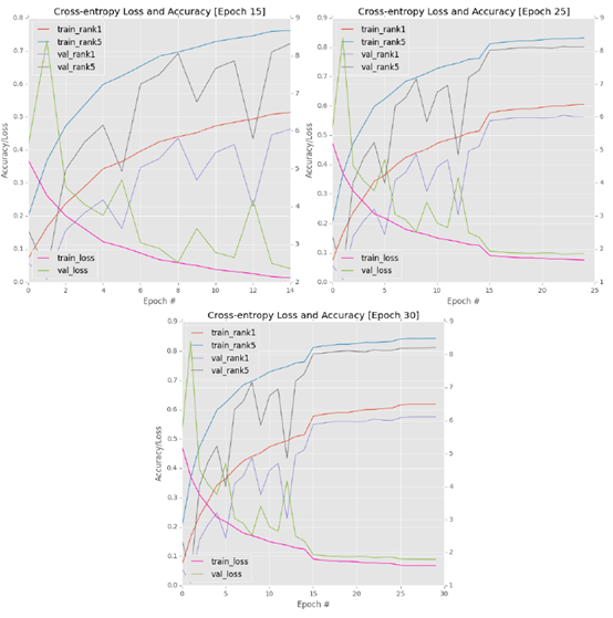Top left: the first 15 epoch s of training GoogLeNet on ImageNet are highly fluctuating. Upper right: reducing the learning rate by an order of magnitude can stabilize the fluctuation; However, learning will soon stagnate. Bottom: reducing the learning rate to 1e-4 will not improve the results.

As demonstrated by the first 15 epochs, learning is very unstable when checking the verification set (above, upper left corner). As the verification loss increases significantly, the verification accuracy decreases sharply. In order to combat volatility, I stopped training after the 15th epoch, reduced the learning rate to 1e-3, and then resumed training:

This update resulted in a complete stagnation of network performance after a slight improvement in accuracy (figure, upper right corner). To verify that the stagnation is indeed true, I stopped training after the 25th epoch, reduced the learning rate to 1e-4, and then continued training for the other 5 epochs:

As my figure shows, the accuracy is slightly improved because SGD can navigate to areas with low loss, but overall, The training has leveled off (figure, bottom). After epoch30, I terminated the training and carefully reviewed the results. A quick check of the log showed that I achieved 57.75% rank-1 and 81.15% rank-5 accuracy on the verification set. Although this is not a bad start, it is far from what I expected: between the accuracy of AlexNet and VGGNet

3.2 GoogLeNet experiment #2

Considering the extreme fluctuation of 1e-2 learning rate, I decided to restart training completely. This time, I used the basic learning rate of 1e-3 to help smooth the learning process. I used the same network architecture, momentum and L2 regularization as the previous experiments. This method leads to stable learning; However, this process is very slow (below, upper left corner).

As learning began to slow down significantly around epoch 70, I stopped training, reduced the learning rate to 1e-4, and then continued training:

As we expected, we can see a small increase in accuracy and a reduction in loss, but learning again failed to make progress (figure, upper right corner). I asked GoogLeNet to continue epoch80, then stopped training again, and reduced my learning rate by an order of magnitude to 1e-5:

As you can now expect, the result is stagnation (figure, bottom). After the 85th epoch, I completely stopped training. Unfortunately, this experiment performed poorly - I only achieved 53.67% rank-1 and 77.85% rank-5 verification accuracy, which is worse than my first experiment.

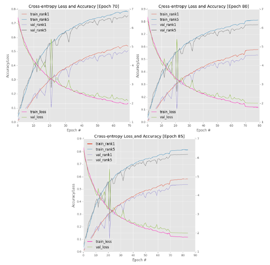Top left: the first 70 periods showed extremely slow but stable learning. Top right: after learning stagnated, I used the SGD optimizer to reduce the learning rate from 1e-3 to 1e-4. However, after the initial turbulence, learning soon stagnated. Bottom: further reducing the learning rate did not improve the results.

3.3 GoogLeNet experiment #3

In view of my experience in using GoogLeNet and Tiny ImageNet in the Practitioner Bundle, I decided to replace Adam's SGD optimizer with an initial (default) learning rate of 1e-3. Using this method, I followed the learning rate decay schedule shown in the table below.

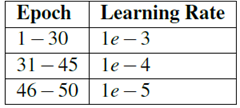
The accuracy and loss diagram is shown in the figure below. Compared with other experiments, We can see that GoogLeNet + Adam quickly achieved a verification accuracy of > 50% (less than 10 epochs, compared with 15 epochs in experiment #1, this is only due to the change of learning rate). It can be seen that reducing the learning rate from 1e-3 to 1e-4 in period 30 introduces an improvement in accuracy. Unfortunately, there is no big jump in period 45. Switch to 1e-5 and continue training five epochs.

After the 50th epoch, stop training. Here, GoogLeNet achieves the accuracy of 63.45% rank-1 and 84.90% rank-5 in the verification set, which is much better than the first two experiments.

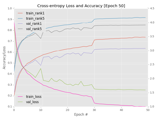When training GoogLeNet, using Adam optimizer produces the best results; However, we cannot replicate the original work of Szegedy et al. Our results are consistent with independent experiments [24], which try to replicate the original performance, but the results are slightly insufficient.

Test the model on the test set:

On the test set, we obtained 65.87% rank-1 and 87.48% rank-5 accuracy. This result is certainly better than AlexNet, but it can not be compared with 71.42% rank-1 and 90.03% rank-5 of VGG.