from sklearn.model_selection import train_test_split


#Divide 30% of the data as the test set

Xtrain, Xtest, Ytrain, Ytest = train_test_split(wine.data, wine.target, test_size=0.3)


clf = DecisionTreeClassifier(random_state=0) #Modeling: Decision Tree

rfc = RandomForestClassifier(random_state=0) #Modeling: random forest


clf = clf.fit(Xtrain, Ytrain) # Training model: Decision Tree

rfc = rfc.fit(Xtrain, Ytrain) # Training model: random forest


score_c = clf.score(Xtest, Ytest) #Return prediction accuracy: random forest

score_r = rfc.score(Xtest, Ytest) #Return prediction accuracy: Decision Tree


# Print out accuracy

print("single Tree:{}".format(score_c),

      "Random Forest:{}".format(score_r))
single Tree:0.9444444444444444 Random Forest:0.9814814814814815
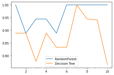
It can be seen that the accuracy of random forest default is higher than that of decision tree.


**4,Draw the effect comparison between random forest and decision tree under a set of cross validation**


> **Cross validation**

> Divide the dataset into n Take each one in turn as the test set n-1 Make a training set and train the model many times to observe the stability of the model
from sklearn.model_selection import cross_val_score
import matplotlib.pyplot as plt
Random forest
rfc = RandomForestClassifier(n_estimators=25)
rfc_s = cross_val_score(rfc, wine.data, wine.target, cv=10)
Decision tree
clf = DecisionTreeClassifier()
clf_s = cross_val_score(clf, wine.data, wine.target, cv=10)
plt.plot(range(1,11), rfc_s, label = "RandomForest")
plt.plot(range(1,11), clf_s, label = "Decision Tree")
plt.legend()
plt.show()
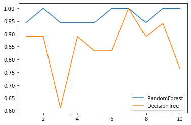
 Another simpler and more interesting way to write:
label = "RandomForest"
for model in [RandomForestClassifier(n_estimators=25),DecisionTreeClassifier()]:
score = cross_val_score(model,wine.data, wine.target, cv=10)

print("{}:".format(label)),print(score.mean())

plt.plot(range(1,11),score,label = label)

plt.legend()

label = "DecisionTree"
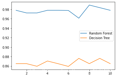
 **5,Draw the effect comparison of random forest and decision tree under ten groups of cross validation**
rfc_l = []
clf_l = []
for i in range(10):
rfc = RandomForestClassifier(n_estimators=25)

rfc_s = cross_val_score(rfc,wine.data,wine.target,cv=10).mean()

rfc_l.append(rfc_s)


clf = DecisionTreeClassifier()

clf_s = cross_val_score(clf,wine.data,wine.target,cv=10).mean()

clf_l.append(clf_s)
plt.plot(range(1,11), rfc_l, label="Random Forest")
plt.plot(range(1,11), clf_l, label="Decision Tree")
plt.legend()
plt.show()
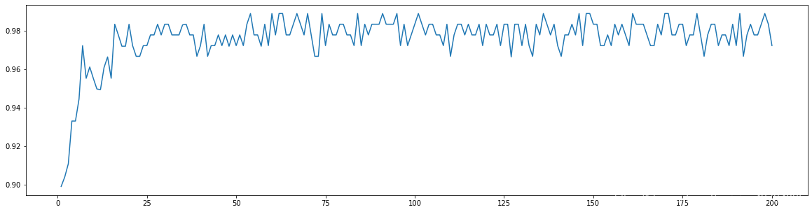
 **6,n\_estimators Learning curve**
#####[TIME WARNING: 2mins 30 seconds]#####
superpa = []
for i in range(200):
rfc = RandomForestClassifier(n_estimators=i+1,n_jobs=-1)

rfc_s = cross_val_score(rfc,wine.data,wine.target,cv=10).mean()

superpa.append(rfc_s)
print(max(superpa), superpa.index(max(superpa))) # 0.9888888888888889 53
plt.figure(figsize=[20,5])
plt.plot(range(1,201),superpa)
plt.show()
 ### []( )random\_state: Controlling the randomness of forest formation patterns > 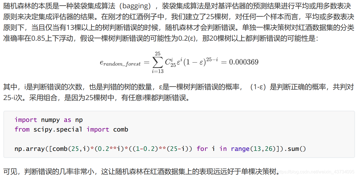 > Think about a question: > We say that the bagged method obeys the majority voting principle or averages the results of the base classifier, which means:**We default that each tree in the forest should be different and will return different results**. > Imagine that if the judgment results of all trees in the random forest are consistent (all right or all wrong), no matter what integration principle is applied to the results, the random forest should**unable**Better results than a single decision tree. But we used the same class DecisionTreeClassifier,With the same parameters, the same training set and test set, why do many trees in the random forest have different judgment results? **In fact, there are in the random forest random\_state**,The usage is similar to that in the classification tree: * In the classification tree, a random\_state Only control the generation of one tree * In random forest random\_state Control is**Patterns of forest formation**,Instead of having only one tree in a forest
rfc = RandomForestClassifier(n_estimators=20, random_state=2)
rfc = rfc.fit(Xtrain, Ytrain)
#One of the important properties of random forest: estimators, to view the status of trees in the forest
rfc.estimators_[0].random_state
for i in range(len(rfc.estimators_)):
print(rfc.estimators_[i].random_state)
We can observe that when random\_state When fixed, a group of fixed trees are generated in the random forest, but each tree is still inconsistent, This is the randomness obtained by the method of "randomly selecting features for branching". And we can prove that when this randomness is greater, the effect of the bagged method will generally be better and better. When the bagged method is used for integration, the base classifiers should be independent and different from each other.
But the limitation of this method is very strong. When we need thousands of trees, the data may not provide thousands of features to let us build as many different trees as possible. Therefore, in addition to random\_state. We need other randomness.
### [](
)bootstrap: Control sampling technique
To make base classifiers as different as possible, an easy way to understand is**Use different training sets for training**,The bagged method forms different training data through the random sampling technology with return,**bootstrap Is the parameter used to control the sampling technique**.
In one containing n A sample of the original training set, we carried out**Random sampling technique with return**:
* One sample is sampled at a time, and the sample is put back into the original training set before the next sample is taken
In other words, this sample may still be collected at the next sampling
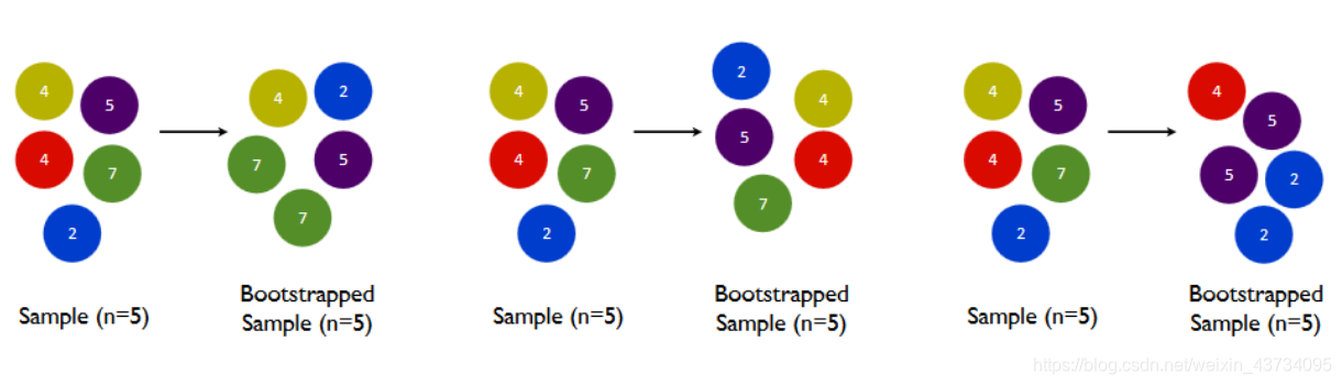
* Such collection n Times, and finally get one as large as the original training set, n Self help set composed of samples
Due to random sampling, the self-service set is different from the original data set and other sampling sets. In this way, we can freely create inexhaustible and different self-help sets. Using these self-help sets to train our base classifiers, our base classifiers will naturally be different.
default`bootstrap=True`,The representative adopts this method**Random sampling technique with return**;Usually not set to False.
[](
)Important attribute
-----------------------------------------------------------------------
### [](
)oob\_score\_: Out of bag data test model accuracy
However, there will also be its own problems with re sampling. Some samples may appear multiple times in the same self-service set, while others may be ignored. Generally speaking, the self-service set contains about 63 samples on average%Raw data. Because the probability of each sample being drawn to a self-service set is:
1 − ( 1 − 1 n ) n 1 - ( 1 - \\frac 1 n)^n 1−(1−n1)n
When n When large enough, this probability converges to 1 − ( 1 e ) 1-(\\frac 1 e) 1−(e1),Approximately equal to 0.632,So there will be about 37%The training data is wasted and not involved in modeling. These data are called**Out of bag data(out of bag data,Abbreviated as oob)**.
When using random forests, we can**Test set and training set are not divided**,use**Out of bag data**To test our model.
Of course, this is not absolute, when n and n\_estimators When they are not big enough, it is likely that no data will fall out of the bag and naturally cannot be used oob Data to test the model.
If you want to test with out of pocket data, you need to set it when instantiating`oob_score=True`. After training, we can use another important attribute of random forest:**oob\_score\_** To view our test results on out of pocket data:
#There is no need to divide the training set and the test set
rfc = RandomForestClassifier(n_estimators=25,oob_score=True)
rfc = rfc.fit(wine.data,wine.target)
#Important attribute oob_score_
rfc.oob_score_
### [](
)estimators\_: Look at the trees in the forest
rfc = RandomForestClassifier(n_estimators=20, random_state=2)
rfc = rfc.fit(Xtrain, Ytrain)
#One of the important properties of random forest: estimators, to view the status of trees in the forest
rfc.estimators_
[](
)Important interfaces: apply,fit,predict,score
-----------------------------------------------------------------------------------------------
The interface of random forest is completely consistent with the decision tree, so there are also four common interfaces: apply,fit,predict,score.
* scoire
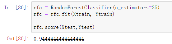
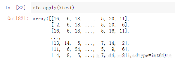
* apply
In addition, we also need to pay attention to the random forest`predict_proba`Interface, which returns the probability that each test sample is assigned to each type of label. If there are several categories of labels, several probabilities are returned.
* If it is a binary problem, then predict\_proba The returned value is greater than 0.5 Is divided into 1 and less than 0.5 , is divided into 0.
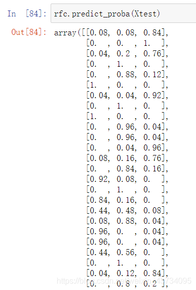
The traditional random forest uses the rules in the bagging method, and the average or minority obeys the majority to determine the integration result sklearn The random forest in is the average corresponding to each sample predict\_proba Return the probability to get an average probability, which determines the classification of test samples.
From the performance of red wine data set, the utility of random forest is much stronger than that of simple decision tree.
[](
)Random forest regressor RandomForestRegressor
================================================================================================
Slightly
[](
)\*The basic idea of parameter adjustment in machine learning
=================================================================================
Most books related to machine learning are about traversing various algorithms and cases to explain the principles and uses of various algorithms, but there is little research on tuning parameters. The main reasons are as follows:
* The method of parameter adjustment is always determined according to the status of the data. There is no way to generalize
* In fact, no one has a particularly good way to adjust parameters
Through painting**learning curve**,perhaps**Grid search**,We can explore the edge of parameter adjustment (the cost may be that it takes three days and three nights to train a model), but in reality, expert parameter adjustment still depends on experience, which comes from:
* Very correct idea and method of parameter adjustment
* Understanding of model evaluation indicators
* Feeling and experience of data
* Try again and again with boundless strength
In machine learning,**A measure of the accuracy of a model on unknown data**be called**Generalization error(Genelization error)**
[](
)\*Generalization error: a measure of the accuracy of a model on unknown data
-------------------------------------------------------------------------------------------
> **Unknown data**: Test set, out of bag data
> When the model is**Unknown data**When the performance is poor, we say that the generalization degree of the model is not enough, the generalization error is large, and the effect of the model is not good.
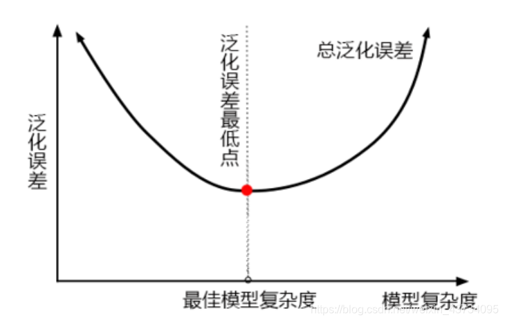
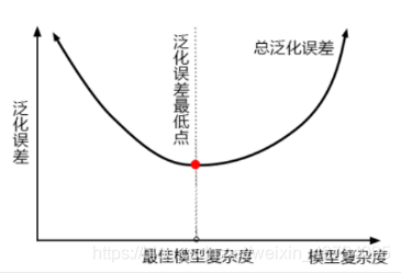
Generalization error is affected by the structure (complexity) of the model. The following figure accurately depicts the relationship between generalization error and model complexity:
* When the model is too**complex**,The model will**Over fitting**,The generalization ability is not enough, so the generalization error is large
* When the model is too**simple**,The model will**Under fitting**,If the fitting ability is not enough, the generalization error will be large
* **Only when the complexity of the model is just good can we achieve the goal of minimizing generalization error**
For the tree model, the more lush the tree, the deeper the depth, and the more branches and leaves, the more complex the model is; Therefore, the tree model is naturally located in the upper right corner of the graph. Random forest is based on tree model, so random forest is also a naturally complex model.
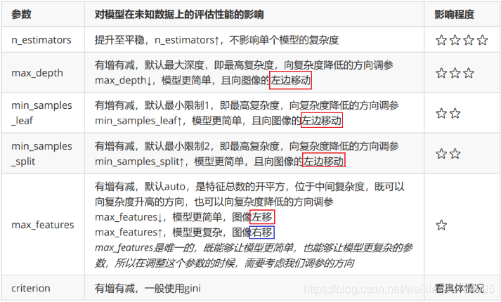
The parameters of random forest are all directed towards one goal:**Reduce the complexity of the model and move the model to the left of the image to prevent over fitting**. Of course, there is no absolute parameter adjustment, and there is also a random forest naturally on the left of the image. Therefore, before adjusting the parameters, we must first judge which side of the image the model is on.
Behind the generalization error is“**deviation-Variance dilemma**",The principle is very complex. We only need to remember four points:
1. If the model is too complex or too simple, the generalization error will be high. What we pursue is the balance point in the middle
2. If the model is too complex, it will over fit, and if the model is too simple, it will under fit
3. For tree model and tree integration model, the deeper the tree is, the more branches and leaves are, and the more complex the model is
4. The goal of tree model and tree integration model is to reduce the complexity of the model and move the model to the left of the image
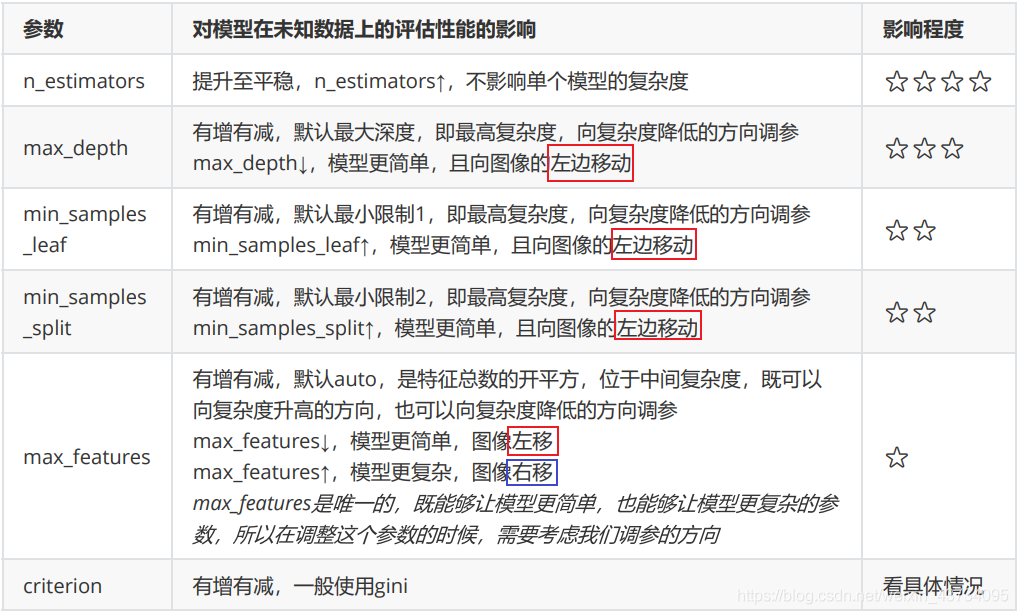
Based on experience, the teacher ranked the impact of various parameters on the model:
With the above knowledge reserves, we can now understand when the model reaches the limit through parameter changes. When the complexity can no longer be reduced, we don't have to adjust it, because adjusting the parameters of large data is very time-consuming and laborious.
In addition to learning curve and grid search, we now have the ability to "speculate" based on the model and correct parameter adjustment ideas, which can make our parameter adjustment ability to a higher level.
[](
)\*\*Example: random forest's adjustment on breast cancer data
========================================================================================
Except that some parameter settings will change during parameter adjustment, other codes are almost the same,**Mainly learn the idea of parameter adjustment!**
Breast cancer data is sklearn One of the self-contained classified data.
**1,Import required libraries**
from sklearn.datasets import load_breast_cancer
from sklearn.ensemble import RandomForestClassifier
from sklearn.model_selection import GridSearchCV
from sklearn.model_selection import cross_val_score
import matplotlib.pyplot as plt
import pandas as pd
import numpy as np
**2,Import datasets and explore data**
data = load_breast_cancer()
data
data.data.shape
data.target
The breast cancer dataset has 569 records and 30 characteristics.
Although the dimension is not too high, the sample size is very small, and over fitting may exist
**3,Conduct a simple modeling to see the effect of the model itself on the dataset**
rfc = RandomForestClassifier(n_estimators=100, random_state=90) # build a random forest of 100 trees, and 90 is lost casually
score_pre = cross_val_score(rfc, data.data, data.target, cv=10).mean() # cross validation
score_pre
Here we can see that the performance of random forests on breast cancer data is pretty good.
In real data sets, it is basically impossible to see an accuracy of more than 95% without adjusting anything
`0.9648809523809524`


**4,The first step of random forest adjustment**: **Adjust first anyway n\_estimators**
"""
Here we select the learning curve. Can we use grid search?
-Yes, but only the learning curve,To see the trend
My personal tendency is to see n_ When did the estimators start to become stable,
Whether the overall accuracy of the model has been promoted,

First learning curve,Can be used to help us delimit the area first,

We take every ten numbers as a stage,To observe n_estimators How does the change of cause the change of the overall accuracy of the model
"""
#####[TIME WARNING: 30 seconds]#####
scorel = []
for i in range(0,200,10):
# Ling n_ estimators = 1,11,21,31..., one hundred and ninety-one

rfc = RandomForestClassifier(n_estimators=i+1,

                             n_jobs=-1,

                             random_state=90)

score = cross_val_score(rfc,data.data,data.target,cv=10).mean() #Cross validation

scorel.append(score) #Every time n_estimators put the accuracy of different cross validation into the score list
#Print the highest cross validation accuracy and its index
#list.index([object]) returns the index of this object in the list
print(max(scorel),(scorel.index(max(scorel))*10)+1)
plt.figure(figsize=[20,5])
plt.plot(range(1,201,10),scorel)
plt.show()
`0.9631265664160402 71` 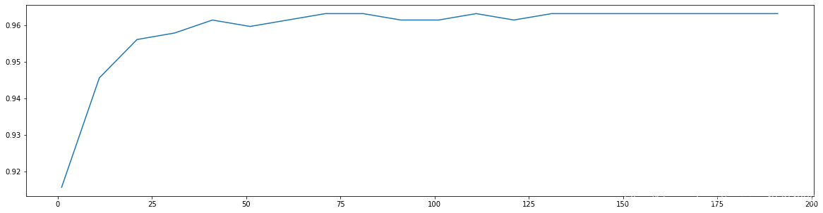 **5,Further refine the learning curve within the range determined in step 4** In step 4, the output has the highest accuracy n\_estimators,The index is 71, so we range it to 65~85
scorel = []
for i in range(64,84):
# Ling n_ estimators = 65,66,67..., eighty-five

rfc = RandomForestClassifier(n_estimators=i+1,

                             n_jobs=-1,

                             random_state=90)

score = cross_val_score(rfc,data.data,data.target,cv=10).mean() #Cross validation

scorel.append(score) #Every time n_estimators put the accuracy of different cross validation into the score list
#Print the highest cross validation accuracy and its index
#list.index([object]) returns the index of this object in the list
print(max(scorel),([*range(64,84)][scorel.index(max(scorel))]))
plt.figure(figsize=[20,5])
plt.plot(range(64,84),scorel)
plt.show()
`0.9666353383458647 72` 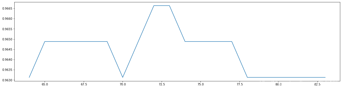 adjustment n\_estimators After that, the accuracy of the model is improved from`0.963...`here we are`0.966...`. Next, we will enter the grid search. We will use the grid search to adjust the parameters one by one. > Why don't we adjust multiple parameters at the same time? There are two reasons: > > 1. Adjusting multiple parameters at the same time will**It runs very slowly**,We don't have so much time in class. > 2. **Adjusting multiple parameters at the same time will make us unable to understand how the combination of parameters comes from**,Even if the results of grid search are bad, we don't know where to change them. Here, in order to use complexity-Generalized error method (variance)-Deviation method), we adjust the parameters one by one. **6,Prepare for grid search and write the parameters of grid search**
"""
Some parameters are not referenced, so it is difficult to specify a range. In this case, we use the learning curve to see the trend
Select a smaller interval from the results of curve running, and then run the curve
param_grid = {'n_estimators':np.arange(0, 200, 10)}
param_grid = {'max_depth':np.arange(1, 20, 1)}
For large data sets, you can try to build from 1000. First enter 1000, an interval for every 100 leaves, and then gradually narrow the range
param_grid = {'max_leaf_nodes':np.arange(25,50,1)}
Some parameters can find a range, or we know their values and values
With their values, how the overall accuracy of the model will change, so we can directly run the grid search
param_grid = {'criterion':['gini', 'entropy']}
param_grid = {'min_samples_split':np.arange(2, 2+20, 1)}
param_grid = {'min_samples_leaf':np.arange(1, 1+10, 1)}
param_grid = {'max_features':np.arange(5,30,1)}
"""
**7,Start to adjust the parameters according to the impact of parameters on the overall accuracy of the model. First, adjust the parameters max\_depth** > According to the table summarized above, we can start from the most influential parameters
#Adjust max_depth
param_grid = {'max_depth':np.arange(1, 20, 1)}
Generally based on the size of the data to carry out a test, breast cancer data is very small, so you can use 110, or 120 of such a test.
However, for large data like digital recognition, we should try 30 ~ 50 layers of depth (maybe not enough)
We should draw a learning curve to observe the influence of depth on the model
rfc = RandomForestClassifier(n_estimators=39,
random_state=90)
GS = GridSearchCV(rfc,param_grid,cv=10)
GS.fit(data.data,data.target)
GS.best_params_
```
`{'max_depth': 6}`
```
GS.best_score_
```
`0.9631265664160402`
**Here, we note that the adjustment max\_depth After that, the accuracy of the model decreased**
* limit max\_depth,To simplify the model, push the model to the left, and the overall accuracy of the model decreases, that is, the overall generalization error increases, which shows that the model is now located on the left of the image, that is**Left of the lowest point of generalization error**(Deviation dominated side)
> Generally speaking,**The random forest should be to the right of the lowest generalization error**,The tree model should tend to over fit rather than under fit; However, this is related to the data set itself, and it may also be adjusted by us n\_estimators It is too large for the data set, so the model is pulled to the lowest point of generalization error. However, since we pursue the minimum generalization error, we keep this n\_estimators,Unless there are other factors that can help us achieve higher accuracy.
When the model is on the left side of the image, what we need is the option to increase the complexity of the model (increase variance and reduce deviation) max\_depth It should be as big as possible, min\_samples\_leaf and min\_samples\_split Should be as small as possible.
This is almost an illustration, except max\_features,We don't have any parameters to adjust because max\_depth,min\_samples\_leaf and min\_samples\_split Is a pruning parameter and a parameter to reduce complexity.
> 
Here, we can predict that we are very close to the upper limit of the model, and the model may not be able to make further progress.
Let's adjust it max\_features,See how the model changes.