Reference link: Mathematical Principles of PCA
Reference link: Understanding PCA and SVD with numpy
Preface
It is well known that the complexity of many machine learning algorithms is closely related to the dimensionality of the data, even exponentially. It is not uncommon to process tens of thousands or even hundreds of thousands of dimensions in real machine learning. In this case, the resource consumption of machine learning is unacceptable, so we must reduce the dimensions of the data. Dimension reduction technology can be divided into supervised and unsupervised ways. Share my understanding of unsupervised dimension reduction PCA today. If there are any inaccuracies, please correct them.
1. Principles and optimization objectives of PCA
PCA is the abbreviation of principal component analysis in order to find some of the major components in the data and discard some of the useless information? How can I know what is useless information? First, let's see what PCA does: The basic idea of PCA is to project the original feature data in some directions so that the projected values are as dispersed as possible, so that the maximum information is retained. Reducing two-dimensional data to one dimension means projecting two-dimensional data onto one dimension, with the projection values as dispersed as possible, so that one-dimensional data may represent two-dimensional data the most. These questions need to be portrayed:
- What is projection?
- How to project?
- How do you characterize projected values as dispersed as possible?
Therefore, the above questions are explained first.
1. What is projection?

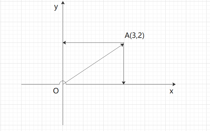
As shown in figure A above, (3,2) means that the OA vector is projected to 4 on the x-axis and 2 on the y-axis.
2. How to project?
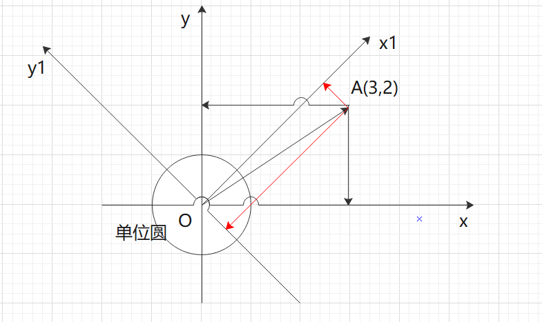
One hidden variable is the base, which the default Cartesian coordinate system is based on (1,0), (0,1), so the linear form of vector OA can be expressed as:

If the coordinate system of a vector becomes x1oy1, then the base of x1oy1 becomes 1/2 of the root sign, and the coordinate of A under the new base is:


Generally, if we have M N-dimensional vectors and want to transform them into a new space represented by R N-dimensional vectors, then first R bases are formed into matrix A by rows, and then vectors are formed into matrix B by columns, then the product AB of the two matrices is the result of the transformation, where the m-th of AB is listed as the result of the m-th column transformation in A.

Finally, the above analysis also finds a physical explanation for matrix multiplication:
Multiplication of two matrices means that each column vector in the right matrix is transformed into the space represented by the base of each row vector in the left matrix.
3. How do you describe projection values as dispersed as possible?
Use Mathematical Principles of PCA Referring to the example in: Covariance Matrix and Optimization Goal_Variance_Covariance_Covariance Matrix_Covariance Matrix Diagonal Reading, the flow of PCA algorithm is as follows:
There are m bars of n-dimensional data.
1) Form the original data into an n-row m-column matrix X by column, that is, transpose the original data
2) Zero-mean each line of X (representing an attribute field), that is, subtract the mean of this line
3) Find the covariance matrix C=1/mXXT**(m is the number of samples, that is, n)**
4) Find the eigenvalues and corresponding eigenvectors of the covariance matrix
5) Arrange the eigenvectors into a matrix in rows from top to bottom according to their corresponding eigenvalue sizes, and take the first k rows to form a matrix P
6) Y=PX is the data after dimension reduction to k. (Note that X is 0-means, not the original data)
2. Mathematical Principles of PCA Pthon implementation of PCA instance in
The PCA algorithm code is as follows:
# -*- coding:utf-8 -*-
import numpy as np
"""
# Original Link: http://blog.codinglabs.org/articles/pca-tutorial.html
PCA The calculation flow of the algorithm:
Set up m strip n Vector Data
1.Compose raw data in columns n That's ok m Column Matrix x,(That is, to transpose the original)
2.take x Zero mean for each row
3.Find the mean of covariance C=1/mXXT(m Is the property of the sample, that is n)
4.Finding the eigenvalues and corresponding eigenvectors of the covariance matrix
5.Arrange the eigenvectors into a matrix from top to bottom according to their corresponding eigenvalue sizes. k Rows make up a projection matrix
6.Y=PX Dimension reduction to k Data for,(X 0-means, not raw data)
"""
def mypca(x,n):
    """
    Function function: Pass in raw data matrix x And final dimension n,Return Projection Matrix p
    """
    # 2. Zero-mean each line of x
    # Average by column
    x = x.T
    x_ = x.mean(axis=1)
    # Dimension decreases after column mean, so dimension elevation is required
    x_ = np.expand_dims(x_, axis=1)
    x = x - x_
    #print(x)
    #[[-1. -1.  0.  2.  0.]
    # [-2.  0.  0.  1.  1.]]
    # 3. Find the covariance mean C=1/mXXT
    c = 1/(x.shape[1])*np.dot(x,x.T)
    #print(c)
    #[[1.2 0.8]
    # [0.8 1.2]]
    # 4. Find the eigenvalues of the covariance matrix and the corresponding eigenvectors
    eig_values,eig_vocter = np.linalg.eig(c)
    #print(eig_values)
    #[2.  0.4]
    #print(eig_vocter)
    #[[ 0.70710678 -0.70710678]
    # [ 0.70710678  0.70710678]]
    # 5. Arrange the eigenvectors into a matrix from top to bottom according to their corresponding eigenvalue sizes, and take k rows to form a projection matrix.
    sort_index = np.argsort(eig_values)[::-1]
    p = eig_vocter[:,sort_index[0:n]]
    #print(p)
    #[0.70710678, 0.70710678]
    return p.T,x

if __name__ == "__main__":

    # 5 pieces of data
    x1 = [1,1]
    x2 = [1,3]
    x3 = [2,3]
    x4 = [4,4]
    x5 = [2,4]
    # 1. Form the original data into an n-row m-column matrix x by column
    x = np.array([x1,x2,x3,x4,x5])
    p,xxx = mypca(x,1)
    x_new = np.dot(p,xxx)
    # [[-2.12132034 -0.70710678  0.          2.12132034  0.70710678]]
    # To accommodate the return format of sklean processing data, a transpose is required
    print(x_new.T)
    #[[-2.12132034]
    #[-0.70710678]
    #[ 0.        ]
    #[ 2.12132034]
    #[ 0.70710678]]
3. Call PCA in sklean to verify PCA, Iris dataset to verify
# -*- coding:utf-8 -*-
import numpy as np
from sklearn.decomposition import PCA
"""
# Original Link: http://blog.codinglabs.org/articles/pca-tutorial.html
PCA The calculation flow of the algorithm:
Set up m strip n Vector Data
1.Compose raw data in columns n That's ok m Column Matrix x,(That is, to transpose the original)
2.take x Zero mean for each row
3.Find the mean of covariance C=1/mXXT(m Is the property of the sample, that is n)
4.Finding the eigenvalues and corresponding eigenvectors of the covariance matrix
5.Arrange the eigenvectors into a matrix from top to bottom according to their corresponding eigenvalue sizes. k Rows make up a projection matrix
6.Y=PX Dimension reduction to k Data for,(X 0-means, not raw data)
"""
def mypca(x,n):
    """
    Function function: Pass in raw data matrix x And final dimension n,Return Projection Matrix p
    """
    # 2. Zero-mean each line of x
    # Average by column
    x = x.T
    x_ = x.mean(axis=1)
    # Dimension decreases after column mean, so dimension elevation is required
    x_ = np.expand_dims(x_, axis=1)
    x = x - x_
    #print(x)
    #[[-1. -1.  0.  2.  0.]
    # [-2.  0.  0.  1.  1.]]
    # 3. Find the covariance mean C=1/mXXT
    c = 1/(x.shape[1])*np.dot(x,x.T)
    #print(c)
    #[[1.2 0.8]
    # [0.8 1.2]]
    # 4. Find the eigenvalues of the covariance matrix and the corresponding eigenvectors
    eig_values,eig_vocter = np.linalg.eig(c)
    #print(eig_values)
    #[2.  0.4]
    #print(eig_vocter)
    #[[ 0.70710678 -0.70710678]
    # [ 0.70710678  0.70710678]]
    # 5. Arrange the eigenvectors into a matrix from top to bottom according to their corresponding eigenvalue sizes, and take k rows to form a projection matrix.
    sort_index = np.argsort(eig_values)[::-1]
    p = eig_vocter[:,sort_index[0:n]]
    #print(p)
    #[0.70710678, 0.70710678]
    return p.T,x

if __name__ == "__main__":

    # 5 pieces of data
    x1 = [1,1]
    x2 = [1,3]
    x3 = [2,3]
    x4 = [4,4]
    x5 = [2,4]
    # 1. Form the original data into an n-row m-column matrix x by column
    x = np.array([x1,x2,x3,x4,x5])
    p,xxx = mypca(x,1)
    x_new = np.dot(p,xxx)
    # [[-2.12132034 -0.70710678  0.          2.12132034  0.70710678]]
    # To accommodate the return format of sklean processing data, a transpose is required
    print(x_new.T)
    #[[-2.12132034]
    #[-0.70710678]
    #[ 0.        ]
    #[ 2.12132034]
    #[ 0.70710678]]
    # Call pca in sklean to verify results
    pca111 = PCA(n_components=1)
    newx = pca111.fit_transform(x)
    print(newx)
    #[[ 2.12132034]
    # [ 0.70710678]
    # [-0.        ]
    # [-2.12132034]
    # [-0.70710678]]
    # Read Iris data for dimension reduction
    import pandas as pd
    pf = pd.read_csv("iris.csv")
    x1 = pf[['150', '4', 'setosa', 'versicolor']].values
    p,xxx1 = mypca(x1,2)
    x1_new = np.dot(p,xxx1)
    # To accommodate the return format of sklean processing data, a transpose is required
    print(x1_new.T[:5,:])
    print("----------------------")
    pca111 = PCA(n_components=2)
    newx = pca111.fit_transform(x1)
    print(newx[:5,:])
[[-2.12132034]
 [-0.70710678]
 [ 0.        ]
 [ 2.12132034]
 [ 0.70710678]]
[[ 2.12132034]
 [ 0.70710678]
 [-0.        ]
 [-2.12132034]
 [-0.70710678]]
[[-2.68412563 -0.31939725]
 [-2.71414169  0.17700123]
 [-2.88899057  0.14494943]
 [-2.74534286  0.31829898]
 [-2.72871654 -0.32675451]]
----------------------
[[-2.68412563  0.31939725]
 [-2.71414169 -0.17700123]
 [-2.88899057 -0.14494943]
 [-2.74534286 -0.31829898]
 [-2.72871654  0.32675451]]
By observing the results, only the negative sign of some results has changed, but the values after dimension reduction are the same. Why is that? This is because in sklean, singular value decomposition SVD is used to solve PCA (in order to improve efficiency), but the result of singular value decomposition is unique, but the positive and negative of the decomposed U matrix and V matrix can not be unique, as long as they are multiplied together consistently. This is why the negative sign is inconsistent. Detailed reference: Understanding PCA and SVD with numpy
summary
PCA algorithm is a dimension reduction method of unsupervised learning. It only needs eigenvalue decomposition to compress and denoise the data. Therefore, it is widely used in real-world scenarios.
The main advantages of the PCA algorithm are:
1) Only the amount of information needs to be measured by variance, not by factors other than the dataset.
2) Orthogonal among the principal components eliminates the influence of the original data components on each other.
3) The calculation method is simple and the main operation is eigenvalue decomposition, which is easy to implement.
The main drawbacks of the PCA algorithm are:
1) The meanings of each feature dimension of the principal component are fuzzier than those of the original sample.
2) Non-principal components with small variances may also contain important information about the sample differences, as dimension reduction discards may have an impact on subsequent data processing.