@TOC
1 Background description
Normally, the growth process of a company's number of customers in one line of business is similar to the population growth in a region. Generally, it will go through these growth stages, namely, silence, growth, explosion, stability. The trend curve of the whole process conforms to the "S" curve. Taking the number of inquiry customers in the automotive aftermarket as an example, when the penetration rate reaches the upper limit and the loss and retention reaches a balance, the number of customers will maintain a stable level. Based on this premise, we try to fit the growth trend of the number of customers with the logistic growth model.
2 Data Exploratory Analysis
Read the data with python, view the information of the data, see if there is missing data, calculate descriptive statistical indicators of the data, and get a general idea of the distribution of the data. The Python code is as follows:
import pandas as pd

data = pd.read_excel(r'D:\logistic Growth Fitting\High-end mid-end car inquiry customer data.xlsx',engine='openpyxl')
print(data.info())
print(data[['Number of high end car inquiry customers','Number of inquiry customers for mid-range vehicles']].describe())
Run result:
<class 'pandas.core.frame.DataFrame'>
RangeIndex: 59 entries, 0 to 58
Data columns (total 3 columns):
 #   Column    Non-Null Count  Dtype
---  ------    --------------  -----
 0   Month        59 non-null     int64
 1   Number of high-end car inquiry customers 59 non-null     int64
 2   Number of inquiry customers for mid-range vehicles 59 non-null     int64
dtypes: int64(3)
memory usage: 1.5 KB
None
           Number of high end car inquiry customers      Number of inquiry customers for mid-range vehicles
count     59.000000     59.000000
mean   14757.254237  12549.542373
std    12560.147425  13848.859081
min      263.000000     45.000000
25%     2693.500000    830.500000
50%    13423.000000   7604.000000
75%    21892.500000  19858.500000
max    42052.000000  47767.000000
From the results, we can see that there is no missing data, and the data of high-end cars is more stable than that of mid-end cars.
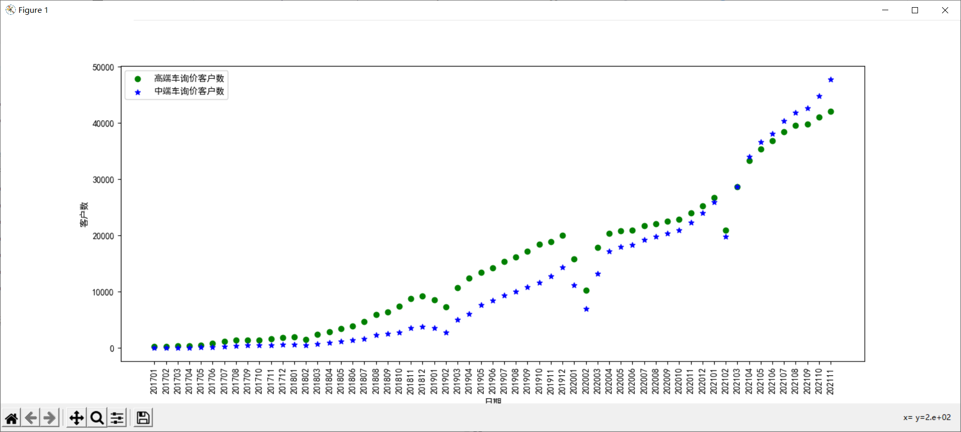
Here we draw a scatter chart to observe the current trend of the number of mid-and high-end car inquiry customers at this stage. The specific python code is as follows:
import matplotlib.pyplot as plt

plt.rcParams['font.sans-serif'] = ['SimHei']    # Solve display problems in Chinese
plt.rcParams['axes.unicode_minus'] = False      # Solving the problem of negative number of coordinate axes

t = data['Month'].to_list()
t1 = np.array(range(1,len(t)+1))

P_A = data['Number of high end car inquiry customers'].values
P_B = data['Number of inquiry customers for mid-range vehicles'].values

# Plot scatterplots
fig1 = plt.figure(figsize=(15,6))
plt.scatter(x=t1,y=P_A,c='g',marker='o',label='Number of high end car inquiry customers')
plt.scatter(x=t1,y=P_B,c='b',marker='*',label='Number of inquiry customers for mid-range vehicles')
plt.xticks(ticks=t1,labels=t,rotation=90)
plt.xlabel('date')
plt.ylabel('Number of customers')
plt.legend(loc=0)
plt.show()
Run result:

As you can see from the picture, due to the influence of the Spring Festival, there has been a cliff drop in the number of inquiry clients in February from 19 to 21 years. Looking at the sample set, there are outliers. If you want to fit the growth rate more accurately, your friends can process the data in February each year. There are two ways to process this: (1) exclude the February data; (2) replace the February data with the arithmetic mean of the three data before February.
3 Model Fitting
Here's a logistic growth model P ( t ) = K P 0 e r ( t − t 0 ) K + P 0 ( e r ( t − t 0 ) − 1 ) P(t)=\frac{KP_0 e^{r(t-t_0)}}{K+P0( e^{r(t-t_0)}-1)} P(t) =K+P 0(er(t_t0) 1) K P 0 er(t_t0) is used as the fitting object to fit the sample data, and the parameters to be estimated are calculated by least squares method. K , P 0 , r K,P_0, r K, P 0, r, where
- t0 is the start time
- K is the environmental capacity, that is, the limit P(t) can reach when growing to the end.
- P0 is the initial capacity, which is the number of times t=0.
- R is the growth rate, the larger r the faster the growth, the faster the approximation to K value, the smaller r the slower the growth, the slower the approximation
The code is as follows:
import numpy as np
from scipy.optimize import curve_fit    # Call this library to fit curves

# Define logistic growth function
def logistic_increase_function(t1, K, P0, r):
    t0 =1
    exp_value = np.exp(r * (t1-t0))
    return (K * exp_value * P0) / (K + (exp_value - 1) * P0)

'''Fitting the number of high-end car inquiry customers'''
# Estimate Fitting Using Least Squares
popt_A, pcov_A = curve_fit(logistic_increase_function, t1, P_A)

# Obtaining fitting coefficients
print("K:capacity  P0:initial_value   r:increase_rate")
print(popt_A)	# [7.91986321e+04 1.85666466e+03 6.59639316e-02]

# Calculate Fit Value
P_A_fit = logistic_increase_function(t1, popt_A[0], popt_A[1], popt_A[2])

'''Fitting the number of mid-end car inquiry customers'''
popt_B, pcov_B = curve_fit(logistic_increase_function, t1, P_B)

# Obtaining fitting coefficients
print("K:capacity  P0:initial_value   r:increase_rate")
print(popt_B)	# [1.20368534e+05 6.55225678e+02 8.25444681e-02]

# Calculate Fit Value
P_B_fit = logistic_increase_function(t1, popt_B[0], popt_B[1], popt_B[2])
You can see that the growth rate of the number of mid-end car inquiry customers is larger than that of high-end cars, which can also be verified by the slope of the scatterplot curve above.
4 Fitting result mapping and future trend prediction
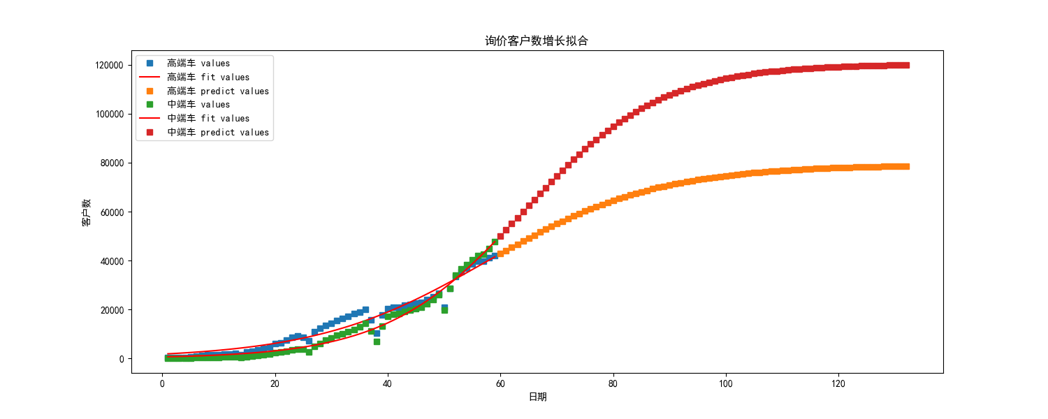
Future trends predict that we will take a little longer to predict when the stability period will be reached, coded as follows:
# Construct a future date list
t_future = [202112] + [i for i in range(202201,202213)] + [i for i in range(202301,202313)] + [i for i in range(202401,202413)] + [i for i in range(202501,202513)] + [i for i in range(202601,202613)] + [i for i in range(202701,202713)]
future = [ i for i in range(t1[-1]+1,t1[-1]+1+len(t_future))]
future = np.array(future)

# Future Forecast
A_future_predict = logistic_increase_function(future, popt_A[0], popt_A[1], popt_A[2])
B_future_predict = logistic_increase_function(future, popt_B[0], popt_B[1], popt_B[2])

# Mapping
fig2 = plt.figure(figsize=(15,6))
plot1_A = plt.plot(t1, P_A, 's', label="High-end cars values",)    # Scatter plot
plot2_A = plt.plot(t1, P_A_fit, 'r', label='High-end cars fit values')    # curve
plot3_A = plt.plot(future, A_future_predict, 's', label='High-end cars predict values')   # Scatter plot
plot1_B = plt.plot(t1, P_B, 's', label="Mid-End Car values",)    # Scatter plot
plot2_B = plt.plot(t1, P_B_fit, 'r', label='Mid-End Car fit values')    # curve
plot3_B = plt.plot(future, B_future_predict, 's', label='Mid-End Car predict values')   # Scatter plot
plt.xlabel('date')
plt.ylabel('Number of customers')
plt.title('Fitting the growth of inquiry customers')
plt.legend(loc=0)  # Specify the lower right corner of the legend position
plt.show()
Drawing results:

From the drawing results, the number of mid-and high-end car inquiry customers of the company is growing, and it is expected to reach a stable period in the first half of 2027.
5 Complete code
import numpy as np
import pandas as pd
from scipy.optimize import curve_fit    # Call this library to fit curves
import matplotlib.pyplot as plt

plt.rcParams['font.sans-serif'] = ['SimHei']    # Solve display problems in Chinese
plt.rcParams['axes.unicode_minus'] = False      # Solving the problem of negative number of coordinate axes

data = pd.read_excel(r'D:\logistic Growth Fitting\High-end mid-end car inquiry customer data.xlsx',engine='openpyxl')
print(data.info())
print(data[['Number of high end car inquiry customers','Number of inquiry customers for mid-range vehicles']].describe())

t = data['Month'].to_list()
t1 = np.array(range(1,len(t)+1))

P_A = data['Number of high end car inquiry customers'].values
P_B = data['Number of inquiry customers for mid-range vehicles'].values

# Plot scatterplots
fig1 = plt.figure(figsize=(15,6))
plt.scatter(x=t1,y=P_A,c='g',marker='o',label='Number of high end car inquiry customers')
plt.scatter(x=t1,y=P_B,c='b',marker='*',label='Number of inquiry customers for mid-range vehicles')
plt.xticks(ticks=t1,labels=t,rotation=90)
plt.xlabel('date')
plt.ylabel('Number of customers')
plt.legend(loc=0)
plt.show()

# Define logistic growth function
def logistic_increase_function(t1, K, P0, r):
    t0 =1
    # t:time   t0:initial time    P0:initial_value    K:capacity  r:increase_rate
    '''
    K For environmental capacity, that is, to grow to the end, P(t)The limit that can be reached.
    P0 For initial capacity, this is t=0 Number of moments.
    r For growth rate, r The larger the growth, the faster the approaching K Value, r The smaller the growth, the slower the approximation
    '''
    exp_value = np.exp(r * (t1-t0))
    return (K * exp_value * P0) / (K + (exp_value - 1) * P0)

'''Fitting the number of high-end car inquiry customers'''
# Estimate Fitting Using Least Squares
popt_A, pcov_A = curve_fit(logistic_increase_function, t1, P_A)

# Obtaining fitting coefficients
print("K:capacity  P0:initial_value   r:increase_rate")
print(popt_A)

# Calculate Fit Value
P_A_fit = logistic_increase_function(t1, popt_A[0], popt_A[1], popt_A[2])

'''Fitting the number of mid-end car inquiry customers'''
popt_B, pcov_B = curve_fit(logistic_increase_function, t1, P_B)

# Obtaining fitting coefficients
print("K:capacity  P0:initial_value   r:increase_rate")
print(popt_B)

# Calculate Fit Value
P_B_fit = logistic_increase_function(t1, popt_B[0], popt_B[1], popt_B[2])

# Construct a future date list
t_future = [202112] + [i for i in range(202201,202213)] + [i for i in range(202301,202313)] + [i for i in range(202401,202413)] + [i for i in range(202501,202513)] + [i for i in range(202601,202613)] + [i for i in range(202701,202713)]
future = [ i for i in range(t1[-1]+1,t1[-1]+1+len(t_future))]
future = np.array(future)

# Future Forecast
A_future_predict = logistic_increase_function(future, popt_A[0], popt_A[1], popt_A[2])
B_future_predict = logistic_increase_function(future, popt_B[0], popt_B[1], popt_B[2])

# Mapping
fig2 = plt.figure(figsize=(15,6))
plot1_A = plt.plot(t1, P_A, 's', label="High-end cars values",)    # Scatter plot
plot2_A = plt.plot(t1, P_A_fit, 'r', label='High-end cars fit values')    # curve
plot3_A = plt.plot(future, A_future_predict, 's', label='High-end cars predict values')   # Scatter plot
plot1_B = plt.plot(t1, P_B, 's', label="Mid-End Car values",)    # Scatter plot
plot2_B = plt.plot(t1, P_B_fit, 'r', label='Mid-End Car fit values')    # curve
plot3_B = plt.plot(future, B_future_predict, 's', label='Mid-End Car predict values')   # Scatter plot
plt.xlabel('date')
plt.ylabel('Number of customers')
plt.title('Fitting the growth of inquiry customers')
plt.legend(loc=0)
plt.show()
Model Fitting Reference Blog: https://blog.csdn.net/weixin_36474809/article/details/104101055/