1 Introduction

1.1 introduction to price demand elasticity

The economics course talks about price demand elasticity, which describes the elasticity of demand quantity with the change of commodity price. Generally, price does not directly affect demand, but is mediated by intermediate variables related to user decision-making. Assuming Q is the quantity demanded by a commodity and P is the price of the commodity, the price elasticity of demand is,

From the above formula, we can simply know that a price change of 1 yuan will lead to greater demand change than a price change of 100 yuan. For example, 100 units of products can be sold every day at the price of 5 yuan. If the price demand elasticity is - 3, the supplier will increase the price by 5% (dp /P, from 5 yuan - > 5.25 yuan), and the demand will decrease by 15% (dQ/Q, from 100 - > 85). Then the income will decrease by 1005-5.2585 = 53.75.
If the unit price decreases by 5%, the income will increase by 46.25. If the supplier knows the price elasticity of the product, it does not need to test repeatedly to know whether the price should be increased or reduced in order to increase revenue.

1.2 start with HEMA counterfactual prediction paper

Before Notes on causal inference -- DML: Double Machine Learning case study (16) This article refers to using DML to calculate price elasticity, but there is no practical operation module. I have read this article Causal inference and counterfactual prediction -- a paper by HEMA KDD2021 (23) After the paper, I want to practice the price elasticity.

Let's first mention the attempt of HEMA on the counterfactual prediction task (how the sales volume changes with the change of discount), semi parametric model, XGBtree model and DeepIV:

• The first is the semi parametric model. However, the semi parametric model for the estimation of sales volume under dynamic discount has not been deeply understood by the author. I feel that the layered price elasticity (average discount tree sales volume prediction + price elasticity fitting dynamic discount sales volume increment) is used to avoid the problem of core causal reasoning. I need to understand the model later
• The second is the wrong attempt, which takes the discount as a treatment and dynamically uses the treatment as a feature to predict the sales volume
• The third, deepIV, takes the average price of three-level categories as an instrument variable

The effect of the three is shown in the figure, and semi para is much better:

This chapter is to enlarge the causal calculation module of price elasticity, which is different from that of HEMA:

• The methods of estimating elasticity are different (this paper uses DML to predict)
• The granularity is different. This case doesn't care about commodity classification. One brain is put together. The elasticity coefficient of HEMA is By each commodity

1.3 DML - price elasticity prediction reasoning steps

The best way, of course, is to directly conduct A/B experiments to test the response of different prices to users' needs, but exogenous factors such as price will directly damage the user experience by showing different prices to different users at the same stage of the same product. Therefore, causal inference is carried out from the observed historical data, but how to control the confounding factors (seasonality, product quality, etc.) is the challenge of causal inference.

Here, DML (Double Machine Learning) method is used for causal inference, which mainly solves two problems:

• First, the important control variables are selected by regularization;
• Second, compared with the traditional linear regression model, nonparametric inference can solve the nonlinear problem.

DML first applies the machine learning algorithm to fit the result variable Y and the processing variable T through the characteristic variables X and W respectively, and then uses the residual of the processing variable to fit the residual of the result variable through the linear model.
The goal is to estimate that the Y function here is the sum of the causal effect of T and the synergistic effect of X and W.

The whole reasoning process of price elasticity in this chapter:

1. The data is divided into two parts. In one part of the samples, the random forest model is selected, and the mixed variables are used to predict the processing variables (price P) to obtain E[P|X]; For other samples, the random forest model can also be selected, and the mixed variables are used to predict the result variable (demand Q) to obtain E[Q|X].

2. Calculate the residuals to obtain the price P and demand Q not affected by hybrid variables, i.e P ~ , Q ~ \widetilde P , \widetilde Q P ,Q ​
   P ~ = P − E [ P ∣ X ] \widetilde P = P-E[P|X] P =P−E[P∣X]
   Q ~ = Q − E [ Q ∣ X ] \widetilde Q = Q-E[Q|X] Q ​=Q−E[Q∣X]

3. Therefore, directly P ~ , Q ~ \widetilde P , \widetilde Q P ,Q The elastic coefficient 𝜃 can be obtained by log log regression:

Need to get θ = d Q ~ / Q ~ d P ~ / P ~ \theta=\frac{d \widetilde Q / \widetilde Q}{d \widetilde P / \widetilde P} θ=dP /P dQ ​/Q ​​

The regression coefficient is obtained by log log regression, i.e l o g Q ~ ～ θ ∗ l o g P ~ + section distance log \widetilde Q ~ \ theta * log \widetilde P + intercept logQ ​～θ∗logP +Intercept

2 case details

Articles associated with this section:

• Causal inference and counterfactual prediction -- a paper by HEMA KDD2021 (23)
• Notes on causal inference -- DML: Double Machine Learning case study (16)

Source of the following case:

• Flexible pricing using machine learning causal reasoning
• Data analysis (29): price demand elasticity and causal inference
• Simple version code: DML.ipynb
• Data set source: Association Rules and Market Basket Analysis

2.1 data cleaning

The data set is kaggle's competition data set. When the original ipynb is directly read in, an error will be reported. Here is a section of kaggle's native reading method, which will not be reported:

data = pd.read_csv('OnlineRetail.csv',encoding= 'cp1252',parse_dates=['InvoiceDate'])
data = data.sort_values(by='InvoiceDate')
data = data.set_index('InvoiceDate')

The original data is shopping basket analysis data. This data set contains all purchase behaviors of a British online retail company during an 8-month period.

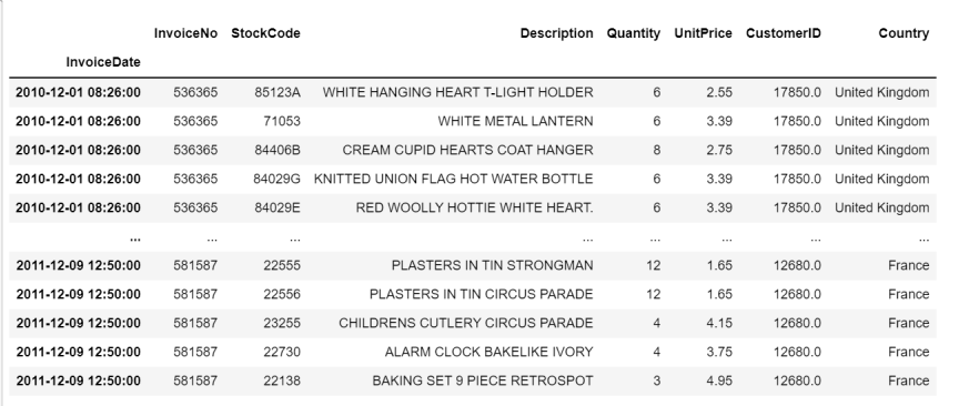
The number of pieces sold per commodity, per country, per store, per time and the corresponding unit price.
Additional processing income is required here:

df['revenue'] = df.Quantity * df.UnitPrice

At the same time, P / Q is logarithmicized:

# log the unit price and quantity
df_mdl = df_mdl.assign(
    LnP = np.log(df_mdl['UnitPrice']),
    LnQ = np.log(df_mdl['Quantity']),
)

2.2 [v1 version] solving price elasticity: OLS regression

v1 version = LnQ~LnP, no covariates, using the simplest OLS regression

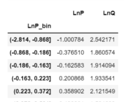
The simplest solution is to segment the lnp and lnQ of the above data, regardless of any causal inference, biased or unbiased. For example (- 2.814, - 0.868) is the average value of lnp and lnQ in this interval, as follows:

The newly generated LnP and LnQ are directly regressed to obtain the regression coefficient:

x='LnP'
y='LnQ'
df = df_mdl
n_bins=15
x_bin = x + '_bin'

df[x_bin] = pd.qcut(df[x], n_bins)

tmp = df.groupby(x_bin).agg({
    x: 'mean',
    y: 'mean'
})
# regression
mdl = sm.OLS(tmp[y], sm.add_constant(tmp[x]))
res = mdl.fit()

Results obtained:

The elasticity coefficient is -0.6064. The higher the price, the less the sales volume

The calculation of v1 can also use another method to calculate the variance,
Because only two variables can:

df_mdl[['LnP', 'LnQ']].cov()

Here is:
θ = − 0.52 0.9 = − 0.60 \theta=\frac{-0.52}{0.9}=-0.60 θ=0.9−0.52​=−0.60

2.3 [v2 version] solving price elasticity: Poisson regression + multiple ridge regression

v2 version = LnQ~LnP+Country+StockCode+Date, with multiple covariates, using ridge regression + Poisson regression

import sklearn.preprocessing
from sklearn import linear_model
from sklearn.pipeline import Pipeline
from sklearn.compose import ColumnTransformer
from sklearn.preprocessing import OneHotEncoder, StandardScaler, RobustScaler
from sklearn.feature_extraction.text import CountVectorizer

feature_generator_basic = ColumnTransformer(
    [
        ('StockCode', OneHotEncoder(), ['StockCode']),
        ('Date', OneHotEncoder(), ['Date']),
        ('Country', OneHotEncoder(), ['Country']),
        ('LnP', 'passthrough', ['LnP']),
    ], remainder='drop'
)

mdl_basic = Pipeline([
    ('feat_proc', feature_generator_basic),
    ('reg', linear_model.PoissonRegressor(
        alpha=1e-6,  # l2 penalty strength; manually selected value for minimum interference on LnP-coef (elasticity)
        fit_intercept=False, # no need, since we have OneHot encodings without drop
        max_iter=100_000, 
    )),
], verbose=True)

mdl_basic_ols = Pipeline([
    ('feat_proc', feature_generator_basic),
    ('reg', linear_model.Ridge(
        alpha=1e-20,  # l2 penalty strength, "very small"
        fit_intercept=False, 
        max_iter=100_000, 
    )),
], verbose=True)

mdl_basic.fit(
    df_mdl[['LnP', 'StockCode', 'Date', 'Country']], 
    df_mdl['Quantity'] # Poisson regression has log-link, so LnQ is implicit in loss function
)

However, the training data is not the same as the previous v1. It does not need to be grouped, and the original data is used directly:

The regression coefficient of LnP in Poisson regression is -2.87559,
The regression coefficient of LnP in Ridge OLS regression is -1.79945,
The results obtained by trying each method vary greatly.

2.4 [v3 version] solving price elasticity: DML

2.4.1 DML data preparation + modeling + residual calculation

Because the unit prices of different products vary greatly, the average unit price of the dimension needs to be subtracted from the unit price of the same dimension:
d L n P i , t = l o g ( p i , t ) − l o g ( p ‾ i ) dLnP_{i,t}=log(p_{i,t})-log(\overline p_{i}) dLnPi,t​=log(pi,t​)−log(p​i​)

Here, the methods to eliminate data differences are as follows:

• Y i o Y_i^\text{o} Yio# is a regular channel product i i i recent average sales
• Y i / Y i nor Y_i/Y_i^\text{nor} Yi / Yinor ， represents the percentage of sales increase caused by the discount price. Because the sales volume of different goods varies greatly, the ratio will be more useful than the absolute value

df_mdl['dLnP'] = np.log(df_mdl.UnitPrice) - np.log(df_mdl.groupby('StockCode').UnitPrice.transform('mean'))
df_mdl['dLnQ'] = np.log(df_mdl.Quantity) - np.log(df_mdl.groupby('StockCode').Quantity.transform('mean'))

Confounding factors were also treated:

1. Seasonal variable: the month in which the price is, the day in the month and the day in the week
2. Duration of product launch: subtract the minimum time of the product from the current time
3. sku price level: the median price within a single sku

df_mdl = df_mdl.assign(
    month = lambda d: d.Date.dt.month,
    DoM =   lambda d: d.Date.dt.day,
    DoW =   lambda d: d.Date.dt.weekday,
    stock_age_days = lambda d: (d.Date - d.groupby('StockCode').Date.transform('min')).dt.days,
    sku_avg_p = lambda d: d.groupby('StockCode').UnitPrice.transform('median')
)

With the confounding factors, LNP and lnq, let's look at the DML process:

• structure l n p − W lnp-W lnp−W， l n q − W lnq-W lnq−W
• Calculate residual

# Confounding factors were modeled separately for Q \ P
model_y = Pipeline([
    ('feat_proc', feature_generator_full),
    ('model_y', RandomForestRegressor(n_estimators=50, min_samples_leaf=3, n_jobs=-1, verbose=0)) 
    # n_samples_leaf/n_estimators is set to reduce model (file) size and runtime
    # larger models yield prettier plots.
])
model_t = Pipeline([
    ('feat_proc', feature_generator_full),
    ('model_t', RandomForestRegressor(n_estimators=50, min_samples_leaf=3, n_jobs=-1, verbose=0))
])

# The estimated value is obtained from the above model
# Get first-step, predictions to residualize ("orthogonalize") with (in-sample for now)
q_hat = model_y.predict(df_mdl)
p_hat = model_t.predict(df_mdl)

# The residual is solved by subtracting the predicted value from the observed value
df_mdl = df_mdl.assign(
    dLnP_res = df_mdl['dLnP'] - p_hat,
    dLnQ_res = df_mdl['dLnQ'] - q_hat,
)

2.4.2 comparison of three models

At this time, after data processing, there are three data types in the dataset:

• logarithm
• Logarithm + de averaging
• Logarithm + de averaging + residual
  
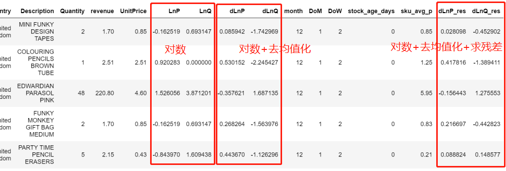
  Then, the three groups of data are segmented according to the processing method of v1 version, and then the price elasticity is calculated by OLS:
  

# Initial ols model
old_fit = binned_ols(
    df_mdl,
    x='LnP',
    y='LnQ',
    n_bins=15,
)
# ols model after initial de averaging
old_fit = binned_ols(
    df_mdl,
    x='dLnP',
    y='dLnQ',
    n_bins=15,
    plot_ax=plt.gca(),
)
# ols model of residual fitting
old_fit = binned_ols(
    df_mdl,
    x='dLnP_res',
    y='dLnQ_res',
    n_bins=15,
    plot_title='Causal regression naively, with item controls, and after DML.',
    plot_ax=plt.gca()
)

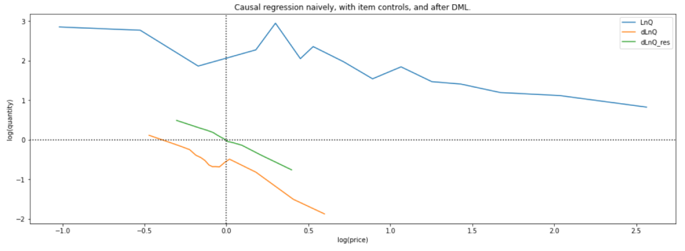
At this time, after data processing, there are three data types in the data set, and the price elasticity of the three is compared:

• logarithm: θ = − 1.7 \theta=-1.7 θ=−1.7
• Logarithm + de averaging: θ = − 1.7 \theta=-1.7 θ=−1.7
• Logarithm + de averaging + residual: θ = − 1.819 \theta=-1.819 θ=−1.819

Of course, OLS also has intercept, which can be obtained from the drawing:

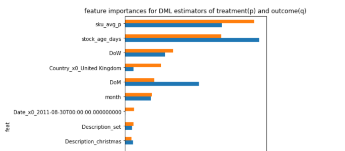
The original text also gives the characteristic importance of two random forest models in the process of DML solution:

feat_imp = pd.DataFrame({
    'feat': get_feat_generator_names(model_y['feat_proc']),
    'importance_q': model_y['model_y'].feature_importances_,
    'importance_p': model_t['model_t'].feature_importances_,
}).set_index('feat')

feat_imp.sort_values(by='importance_p').iloc[-15:].plot.barh(
    figsize=(5, 8), 
    title='feature importances for DML estimators of treatment(p) and outcome(q)'
)

2.4.3 robustness assessment

The main lessons learned in this chapter are as follows:

• A data screening principle, after orthogonalization of residuals, d L n P r e s dLnP_{res} dLnPres # is always small, so in order to reduce noise, we will discard all very small price change observations, which do not contain much information
  The training data is divided into multiple k-fold s to test the stability of the elastic coefficient

Well, take a look at this picture in the article of HEMA,
Use the proportion of training data to the stability distribution of several models

The prediction and inference result of the model is
θ ^ = d L n Q r e s d L n P r e s \hat \theta=\frac{dLnQ_{res}}{dLnP_{res}} θ^=dLnPres​dLnQres​​

But after orthogonalizing the residuals, d L n P r e s dLnP_{res} dLnPres is always small, so in order to reduce noise, we will discard all very small price change observations, which do not contain much information.

Chernozhukov proposes an improved DML, which is estimated by the traditional standard OLS method
θ ^ = ( P ~ T P ~ ) − 1 P ~ T Q ~ \hat \theta=(\widetilde P^T \widetilde P)^{-1}\widetilde P^T \widetilde Q θ^=(P TP )−1P TQ ​
But improved
θ ^ = ( P ~ T P ) − 1 P ~ T Q ~ T \hat \theta=(\widetilde P^T P)^{-1}\widetilde P^T \widetilde Q^T θ^=(P TP)−1P TQ ​T
That is, the second P matrix is non residualized.

Finally, the average value is obtained by 2-fold, which makes the result more robust, and the final elastic coefficient is -1.89

old_fit = binned_ols(
    df_mdl,
    x='dLnP',
    y='dLnQ',
    n_bins=15,
    plot_ax=plt.gca(),
)
plt.gca().set(
    xlabel='log(price)',
    ylabel='log(quantity)',    
)
plt.gca().axvline(0, color='k', linestyle=':')
plt.gca().axhline(0, color='k', linestyle=':')


elast_estimates = list()
for idx_aux, idx_inf in KFold(n_splits=2, shuffle=True).split(df_mdl):
    
    df_aux = df_mdl.iloc[idx_aux]
    df_inf = df_mdl.iloc[idx_inf].copy()
    
    # step 1: aux models and residualize in inferential set
    print('fitting model_y')
    model_y.fit(df_aux, df_aux.dLnQ)
    print('fitting model_t')
    model_t.fit(df_aux, df_aux.dLnP)
    
    df_inf = df_inf.assign(
        dLnP_res = df_inf['dLnP'] - model_t.predict(df_inf),
        dLnQ_res = df_inf['dLnQ'] - model_y.predict(df_inf),
    )
    
    binned_ols(
        df_inf,
        x='dLnP_res',
        y='dLnQ_res',
        n_bins=15,
        plot_ax=plt.gca(),
        label='fold'
    )
    
    # ignore observations where we residualized away all variation in price
    mask = (~(df_inf.dLnP_res.abs() < 0.01))
    df_inf_censored = df_inf[mask]
    
    # step 2.1: Chernozhukov DML inference
    elast = (
        df_inf_censored['dLnP_res'].dot(df_inf_censored['dLnQ_res'])
        /
        df_inf_censored['dLnP_res'].dot(df_inf_censored['dLnP'])
        # the last part here deviates from standard OLS solution
    )
    
    print('DML elast: ', elast)
    elast_estimates.append(elast)

    print('OLS elasticity for comparison:',
        df_inf_censored['dLnP_res'].dot(df_inf_censored['dLnQ_res'])
        /
        df_inf_censored['dLnP_res'].dot(df_inf_censored['dLnP_res'])
    )    

print("DML efficient estimate of elasticity:", np.mean(elast_estimates))

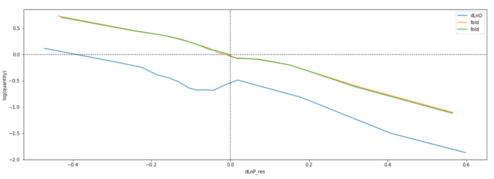
Here, let's compare the article of HEMA, which seems to be comparable to their semi parametric model?