This article is shared from Huawei cloud community< [Python artificial intelligence] 23 Emotion classification based on machine learning and TFIDF (including detailed NLP data cleaning) >, by eastmount.
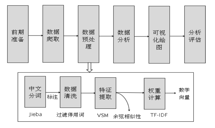
In data analysis and data mining, it usually needs to go through the steps of preliminary preparation, data crawling, data preprocessing, data analysis, data visualization and evaluation analysis. The work before data analysis takes nearly half the working time of data engineers, and the data preprocessing will also directly affect the quality of subsequent model analysis. Figure is the basic steps of data preprocessing, including Chinese word segmentation, part of speech tagging, data cleaning, feature extraction (vector space model storage), weight calculation (TF-IDF), etc.
I Chinese word segmentation
After the reader crawls the Chinese data set using Python, he first needs to perform Chinese word segmentation on the data set. Because words in English are related by spaces, and phrases can be divided directly according to the spaces, word segmentation is not required. Chinese characters are closely connected and have semantics, and there is no obvious separation point between words. Therefore, it is necessary to use Chinese word segmentation technology to segment sentences in the corpus according to spaces into a word sequence. Now let's introduce Chinese word segmentation technology and Jiaba Chinese word segmentation tool in detail.
Chinese Word Segmentation refers to the segmentation of Chinese character sequences into individual word or word string sequences. It can establish separation marks in Chinese strings without word boundaries, usually separated by spaces. Let's take a simple example to segment the sentence "I'm a programmer".
Input: I am a programmer
 Output 1: I\yes\Course\order\member
 Output 2: I am\It's Cheng\program\Sequencer
 Output 3: I\yes\programmer
For example, the code is mainly imported Jieba extension package, and then call its function for Chinese word segmentation.
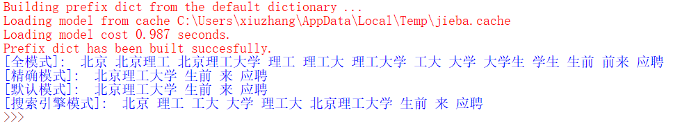
#encoding=utf-8
import jieba

text = "Beijing Polytechnic University students come to apply"

data = jieba.cut(text,cut_all=True)   #Full mode
print("[Full mode]: ", " ".join(data))

data = jieba.cut(text,cut_all=False)  #Precise mode
print("[Precise mode]: ", " ".join(data))

data = jieba.cut(text)  #The default is precise mode
print("[Default mode]: ", " ".join(data))

data = jieba.cut_for_search(text)  #Search engine mode
print("[Search engine mode]: ", " ".join(data))
The above code output is as follows, including the results of full mode, accurate mode and search engine mode output.
II Data cleaning
In the process of analyzing the corpus, there are usually some dirty data or noisy phrases that interfere with our experimental results, which requires Data Cleaning of the corpus after word segmentation. For example, Jieba tool is used for Chinese word segmentation. It may have some dirty data or stop words, such as "we", "de", "do" and so on. These words reduce the data quality. In order to get better analysis results, it is necessary to clean the data set or stop word filtering.
- incomplete data
- Duplicate data
- Error data
- Stop words
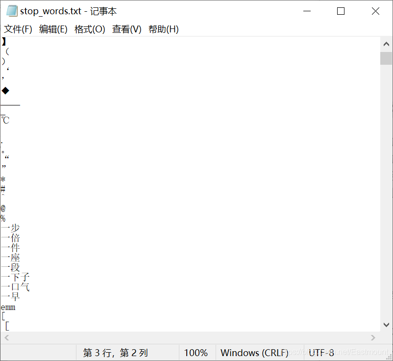
Here we mainly explain the stop word filtering to delete the stop words that occur frequently but do not affect the text topic. Introducing stop in Jieb word segmentation_ words. Txt stop word dictionary. If it exists, filter it.
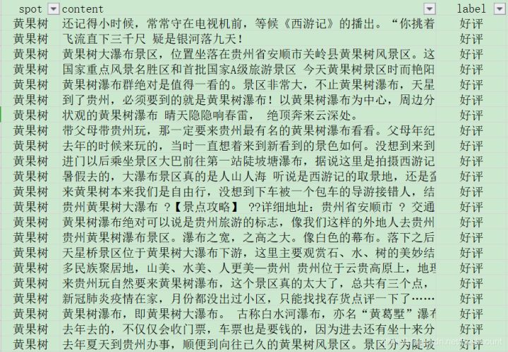
The following is the comment information of "Huangguoshu waterfall" from websites such as public comments and meituan. We use Jieba tool to segment Chinese words.
- Praise: 5000
- Bad comments: 1000
Full code:
# -*- coding:utf-8 -*-
import csv
import pandas as pd
import numpy as np
import jieba
import jieba.analyse

#Add custom dictionaries and deactivate Dictionaries
jieba.load_userdict("user_dict.txt")
stop_list = pd.read_csv('stop_words.txt',
                        engine='python',
                        encoding='utf-8',
                        delimiter="\n",
                        names=['t'])['t'].tolist()

#Chinese word segmentation function
def txt_cut(juzi):
    return [w for w in jieba.lcut(juzi) if w not in stop_list]

#Write word segmentation results
fw = open('fenci_data.csv', "a+", newline = '',encoding = 'gb18030')
writer = csv.writer(fw)
writer.writerow(['content','label'])

# Using CSV Dictreader reads the information in the file
labels = []
contents = []
file = "data.csv"
with open(file, "r", encoding="UTF-8") as f:
    reader = csv.DictReader(f)
    for row in reader:
        # Data element acquisition
        if row['label'] == 'Praise':
            res = 0
        else:
            res = 1
        labels.append(res)
        content = row['content']
        seglist = txt_cut(content)
        output = ' '.join(list(seglist))            #Space splicing
        contents.append(output)

        #File write
        tlist = []
        tlist.append(output)
        tlist.append(res)
        writer.writerow(tlist)

print(labels[:5])
print(contents[:5])
fw.close()
The running results are shown in the figure below. On the one hand, it filters special punctuation marks and stop words, and on the other hand, it imports user_dict.txt dictionary divides proper nouns such as "Huangguoshu waterfall" and "scenic spot", otherwise it may be divided into "Huangguoshu" and "waterfall", "scenery" and "scenic spot".
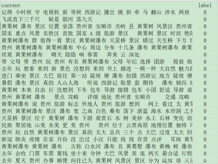
- Before data cleaning
I still remember when I was a child, I often stood in front of the TV, waiting for the broadcast of journey to the West. "You carry the load, I lead the horse. Climb the mountain, wade in the water and slide on both shoulders "The familiar song sounded in our ears again. The water in the lyrics is the water in Guizhou. To be exact, it is the Huangguoshu waterfall in Guizhou. That waterfall flows into our childhood and makes us linger. Huangguoshu waterfall is not only a waterfall, but a large scenic spot, including steep slope pond waterfall, Tianxing bridge scenic spot and Huangguoshu waterfall, among which Huangguoshu Falls The great waterfall is the most famous.
- After data cleaning
I remember when I was a child, I waited in front of the TV for the broadcast of journey to the West. I carried my horse across the mountain and waded across the water. I was familiar with the song. When the song sounded, the water level in the lyrics did say that the curtain of Huangguoshu waterfall in Guizhou flowed into my childhood. Huangguoshu Waterfall Scenic Spot includes steep slope pond waterfall Tianxing bridge scenic spot Huangguoshu waterfall Huangguoshu waterfall name
III Feature extraction and TF-IDF calculation
1. Basic concepts
Weight calculation is to measure the importance of feature items in document representation through feature weight, and give feature words a certain weight to measure and count text feature words. TF-IDF (term frequency inverters document frequency) is a classical weight calculation technology used in data analysis and information processing in recent years. This technology calculates the importance of the feature word in the whole corpus according to the number of times the feature word appears in the text and the document frequency in the whole corpus. Its advantage is that it can filter out some common but insignificant words and retain as many feature words with high influence as possible.
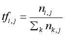
The calculation formula of TF-IDF is as follows, where TF-IDF represents the product of word frequency TF and inverted text word frequency IDF. The weight in TF-IDF is directly proportional to the frequency of feature items in documents and inversely proportional to the number of documents in the whole corpus. The larger the TF-IDF value, the higher the importance of the feature word to the text.
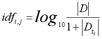
Among them, the calculation formula of TF word frequency is as follows. Ni and j are the times that the feature word ti appears in the training text Dj, and the denominator is the number of all feature words in the text Dj. The calculation result is the word frequency of a feature word.
Inverse Document Frequency (IDF) is a classical method proposed by Spark Jones in 1972 to calculate the weight of words and documents. The calculation formula is as follows. The parameter | D | represents the total number of texts in the corpus, and | Dt | represents the number of feature words tj contained in the text.
In the inverse document frequency method, the weight changes inversely with the number of documents of feature words. For example, some common words such as "we", "but" and "de" appear frequently in all documents, but their IDF value is very low. Even if it appears in every document, the calculation result of log1 is 0, which reduces the role of these common words; On the contrary, if a word introducing "artificial intelligence" appears only many times in the document, its function is very high.
The core idea of TF-IDF technology is that if a feature word appears frequently in one article and rarely in other articles, it is considered that this word or phrase has good classification ability and is suitable for weight calculation. TF-IDF algorithm is simple and fast, and the results are also in line with the actual situation. It is a common means in the fields of text mining, emotion analysis, topic distribution and so on.
2. Code implementation
Scikit learn mainly uses two classes in scikit learn, CountVectorizer and TfidfTransformer, to calculate word frequency and TF-IDF value.
- CountVectorizer
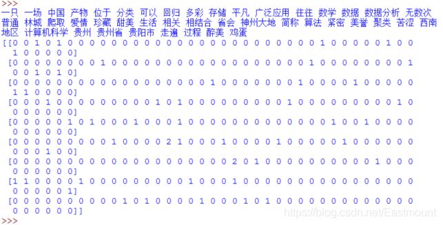
This class is to convert text words into the form of word frequency matrix. For example, the text "I am a teacher" contains four words. The word frequency of their corresponding words is 1, and "I", "am", "a" and "teacher" appear once respectively. CountVectorizer will generate a matrix a[M][N], a total of M text corpora and N words. For example, a[i][j] represents the word frequency of word j under class I text. Then call fit_ The transform() function calculates the number of occurrences of each word, get_ feature_ The names () function gets all text keywords in the thesaurus.
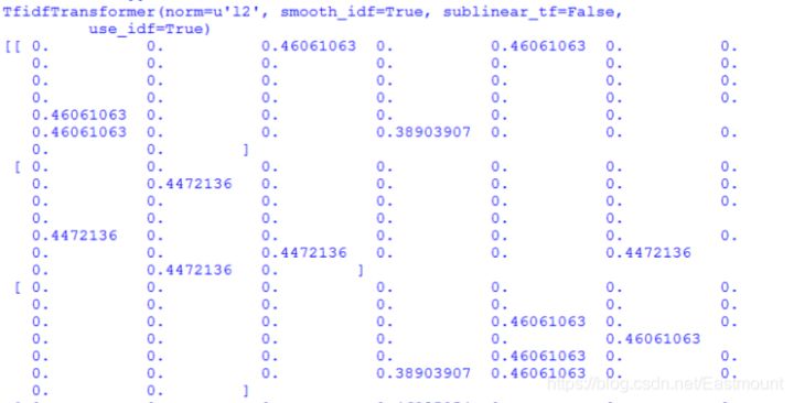
- TfidTransformer
After the word frequency matrix is calculated using the CountVectorizer class, the TF-IDF value of each word in the vectorizer variable is counted through the TfidfTransformer class. TF-IDF values are stored in the form of matrix array. Each row of data represents a text corpus, and each column of each row represents the weight corresponding to one of the features. After TF-IDF is obtained, various data analysis algorithms can be used for analysis, such as cluster analysis, LDA topic distribution, public opinion analysis, etc.
Full code:
# -*- coding:utf-8 -*-
import csv
import pandas as pd
import numpy as np
import jieba
import jieba.analyse
from scipy.sparse import coo_matrix
from sklearn import feature_extraction
from sklearn.feature_extraction.text import TfidfVectorizer
from sklearn.feature_extraction.text import CountVectorizer
from sklearn.feature_extraction.text import TfidfTransformer

#----------------------------------Step 1: read the file--------------------------------
with open('fenci_data.csv', 'r', encoding='UTF-8') as f:
    reader = csv.DictReader(f)
    labels = []
    contents = []
    for row in reader:
        labels.append(row['label']) #0-Praise 1-negative comment
        contents.append(row['content'])

print(labels[:5])
print(contents[:5])

#----------------------------------Step 2 data preprocessing--------------------------------
#Convert the words in the text into word frequency matrix. The matrix element a[i][j] represents the word frequency of j words under class I text
vectorizer = CountVectorizer()

#This class will count the tf of each word-idf Weight
transformer = TfidfTransformer()

#First fit_transform is the calculation of tf-idf the second fit_transform Is to convert text into word frequency matrix
tfidf = transformer.fit_transform(vectorizer.fit_transform(contents))
for n in tfidf[:5]:
    print(n)
print(type(tfidf))

# Get all words in the word bag model
word = vectorizer.get_feature_names()
for n in word[:10]:
    print(n)
print("Number of words:", len(word))

#Will tf-idf Matrix extraction, elements w[i][j]express j Word in i In class text tf-idf weight
#X = tfidf.toarray()
X = coo_matrix(tfidf, dtype=np.float32).toarray() #Sparse matrix note float
print(X.shape)
print(X[:10])
The output results are as follows:
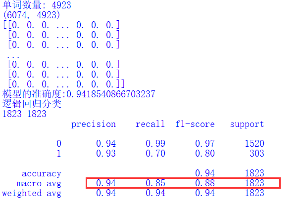
<class 'scipy.sparse.csr.csr_matrix'>
aaaaa
achievements
amazing
ananananan
ancient
anshun
aperture
app

Number of words: 20254
(6074, 20254)
[[0. 0. 0. ... 0. 0. 0.]
 [0. 0. 0. ... 0. 0. 0.]
 [0. 0. 0. ... 0. 0. 0.]
 ...
 [0. 0. 0. ... 0. 0. 0.]
 [0. 0. 0. ... 0. 0. 0.]
 [0. 0. 0. ... 0. 0. 0.]]
3.MemoryError memory overflow error
When we have a large amount of data, the matrix can not store such a large amount of data, and the following errors will occur:
- ValueError: array is too big; arr.size * arr.dtype.itemsize is larger than the maximum possible size.
- MemoryError: Unable to allocate array with shape (26771, 69602) and data type float64
My solutions are as follows:
- Stop word filtering reduces unwanted feature words
- The scipy package provides the creation of sparse matrix, using coo_matrix(tfidf, dtype=np.float32) converts tfidf
- CountVectorizer(min_df=5) increases min_ DF parameter, which filters out feature words with less frequency. This parameter can be debugged continuously
max_df is used to delete terms that appear too frequently. It is called corpus specific stop words. The default is max_df is 1.0, which ignores terms that appear in 100% of documents; min_df is used to delete the infrequent term min_df=5 means ignoring terms that appear in less than 5 documents. - Use GPU or expand memory to solve
IV Emotion classification based on logistic regression
After obtaining the text TF-IDF value, this section briefly explains the process of emotion classification using TF-IDF value, mainly including the following steps:
- Generate word frequency matrix for Chinese word segmentation and data cleaned corpus. It mainly calls the CountVectorizer class to calculate the word frequency matrix, and the generated matrix is X.
- Call the TfidfTransformer class to calculate the TF-IDF value of word frequency matrix X to obtain the Weight matrix.
- Call Sklearn machine learning package to perform classification operation, call fit() function for training, and assign the predicted class mark to the pre array.
- Call the PCA() function of Sklearn library to reduce the dimension, reduce these features to two dimensions, corresponding to the X and Y axes, and then visually present them.
- Algorithm optimization and algorithm evaluation.
Complete code of logistic regression:
# -*- coding:utf-8 -*-
import csv
import pandas as pd
import numpy as np
import jieba
import jieba.analyse
from scipy.sparse import coo_matrix
from sklearn import feature_extraction
from sklearn.feature_extraction.text import TfidfVectorizer
from sklearn.feature_extraction.text import CountVectorizer
from sklearn.feature_extraction.text import TfidfTransformer
from sklearn.model_selection import train_test_split
from sklearn.metrics import classification_report
from sklearn.linear_model import LogisticRegression
from sklearn.ensemble import RandomForestClassifier
from sklearn.tree import DecisionTreeClassifier
from sklearn import svm
from sklearn import neighbors
from sklearn.naive_bayes import MultinomialNB

#----------------------------------Step 1: read the file--------------------------------
with open('fenci_data.csv', 'r', encoding='UTF-8') as f:
    reader = csv.DictReader(f)
    labels = []
    contents = []
    for row in reader:
        labels.append(row['label']) #0-Praise 1-negative comment
        contents.append(row['content'])

print(labels[:5])
print(contents[:5])

#----------------------------------Step 2 data preprocessing--------------------------------
#Convert the words in the text into word frequency matrix. The matrix element a[i][j] represents the word frequency of j words under class I text
vectorizer = CountVectorizer(min_df=5)

#This class will count the tf of each word-idf Weight
transformer = TfidfTransformer()

#First fit_transform is the calculation of tf-idf the second fit_transform Is to convert text into word frequency matrix
tfidf = transformer.fit_transform(vectorizer.fit_transform(contents))
for n in tfidf[:5]:
    print(n)
print(type(tfidf))

# Get all words in the word bag model
word = vectorizer.get_feature_names()
for n in word[:10]:
    print(n)
print("Number of words:", len(word))

#Will tf-idf Matrix extraction, elements w[i][j]express j Word in i In class text tf-idf weight
#X = tfidf.toarray()
X = coo_matrix(tfidf, dtype=np.float32).toarray() #Sparse matrix note float
print(X.shape)
print(X[:10])

#----------------------------------Step 3 data division--------------------------------
#Using train_test_split split X y list
X_train, X_test, y_train, y_test = train_test_split(X,
                                                    labels,
                                                    test_size=0.3,
                                                    random_state=1)

#--------------------------------Step 4 machine learning classification--------------------------------
# Logistic regression classification method model
LR = LogisticRegression(solver='liblinear')
LR.fit(X_train, y_train)
print('Accuracy of model:{}'.format(LR.score(X_test, y_test)))
pre = LR.predict(X_test)
print("Logistic regression classification")
print(len(pre), len(y_test))
print(classification_report(y_test, pre))
print("\n")
The operation results are shown in the figure below:
V Algorithm performance evaluation
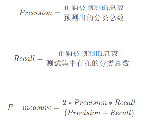
We need to write our own programs to realize many real-time algorithm evaluation, such as drawing ROC curve, counting various characteristic information and displaying 4-digit results. Here, the author tries to customize the accuracy, Recall and F-measure. The calculation formula is as follows:
Since this paper mainly focuses on the problem of 2 classification, the experimental evaluation is mainly divided into 0 and 1. The complete code is as follows:
# -*- coding:utf-8 -*-
import csv
import pandas as pd
import numpy as np
import jieba
import jieba.analyse
from scipy.sparse import coo_matrix
from sklearn import feature_extraction
from sklearn.feature_extraction.text import TfidfVectorizer
from sklearn.feature_extraction.text import CountVectorizer
from sklearn.feature_extraction.text import TfidfTransformer
from sklearn.model_selection import train_test_split
from sklearn.metrics import classification_report
from sklearn.linear_model import LogisticRegression
from sklearn.ensemble import RandomForestClassifier
from sklearn.tree import DecisionTreeClassifier
from sklearn import svm
from sklearn import neighbors
from sklearn.naive_bayes import MultinomialNB

#----------------------------------Step 1: read the file--------------------------------
with open('fenci_data.csv', 'r', encoding='UTF-8') as f:
    reader = csv.DictReader(f)
    labels = []
    contents = []
    for row in reader:
        labels.append(row['label']) #0-Praise 1-negative comment
        contents.append(row['content'])

print(labels[:5])
print(contents[:5])

#----------------------------------Step 2 data preprocessing--------------------------------
#Convert the words in the text into word frequency matrix. The matrix element a[i][j] represents the word frequency of j words under class I text
vectorizer = CountVectorizer(min_df=5)

#This class will count the tf of each word-idf Weight
transformer = TfidfTransformer()

#First fit_transform is the calculation of tf-idf the second fit_transform Is to convert text into word frequency matrix
tfidf = transformer.fit_transform(vectorizer.fit_transform(contents))
for n in tfidf[:5]:
    print(n)
print(type(tfidf))

# Get all words in the word bag model
word = vectorizer.get_feature_names()
for n in word[:10]:
    print(n)
print("Number of words:", len(word))

#Will tf-idf Matrix extraction, elements w[i][j]express j Word in i In class text tf-idf weight
#X = tfidf.toarray()
X = coo_matrix(tfidf, dtype=np.float32).toarray() #Sparse matrix note float
print(X.shape)
print(X[:10])

#----------------------------------Step 3 data division--------------------------------
#Using train_test_split split X y list
X_train, X_test, y_train, y_test = train_test_split(X,
                                                    labels,
                                                    test_size=0.3,
                                                    random_state=1)

#--------------------------------Step 4 machine learning classification--------------------------------
# Logistic regression classification method model
LR = LogisticRegression(solver='liblinear')
LR.fit(X_train, y_train)
print('Accuracy of model:{}'.format(LR.score(X_test, y_test)))
pre = LR.predict(X_test)
print("Logistic regression classification")
print(len(pre), len(y_test))
print(classification_report(y_test, pre))

#----------------------------------Step 5 evaluation results--------------------------------
def classification_pj(name, y_test, pre):
    print("Algorithm evaluation:", name)

    # Accuracy = Total number of correctly identified individuals /  Total number of individuals identified
    # Recall rate = Total number of correctly identified individuals /  Total number of individuals in the test set
    # F value f-measure = Correct rate * recall  * 2 / (Correct rate + recall )

    YC_B, YC_G = 0,0  #Predict bad good
    ZQ_B, ZQ_G = 0,0  #correct
    CZ_B, CZ_G = 0,0  #existence

    #0-good 1-bad At the same time, it is calculated to prevent the change of class standard
    i = 0
    while i<len(pre):
        z = int(y_test[i])   #real
        y = int(pre[i])      #forecast

        if z==0:
            CZ_G += 1
        else:
            CZ_B += 1

        if y==0:
            YC_G += 1
        else:
            YC_B += 1

        if z==y and z==0 and y==0:
            ZQ_G += 1
        elif z==y and z==1 and y==1:
            ZQ_B += 1
        i = i + 1

    print(ZQ_B, ZQ_G, YC_B, YC_G, CZ_B, CZ_G)
    print("")

    # Result output
    P_G = ZQ_G * 1.0 / YC_G
    P_B = ZQ_B * 1.0 / YC_B
    print("Precision Good 0:", P_G)
    print("Precision Bad 1:", P_B)

    R_G = ZQ_G * 1.0 / CZ_G
    R_B = ZQ_B * 1.0 / CZ_B
    print("Recall Good 0:", R_G)
    print("Recall Bad 1:", R_B)

    F_G = 2 * P_G * R_G / (P_G + R_G)
    F_B = 2 * P_B * R_B / (P_B + R_B)
    print("F-measure Good 0:", F_G)
    print("F-measure Bad 1:", F_B)

#function call
classification_pj("LogisticRegression", y_test, pre)
The output results are as follows:
Logistic regression classification
1823 1823
              precision    recall  f1-score   support

           0       0.94      0.99      0.97      1520
           1       0.93      0.70      0.80       303

    accuracy                           0.94      1823
   macro avg       0.94      0.85      0.88      1823
weighted avg       0.94      0.94      0.94      1823

Algorithm evaluation: LogisticRegression
213 1504 229 1594 303 1520

Precision Good 0: 0.9435382685069009
Precision Bad 1: 0.9301310043668122
Recall Good 0: 0.9894736842105263
Recall Bad 1: 0.7029702970297029
F-measure Good 0: 0.9659601798330122
F-measure Bad 1: 0.800751879699248
Vi Algorithm comparison experiment
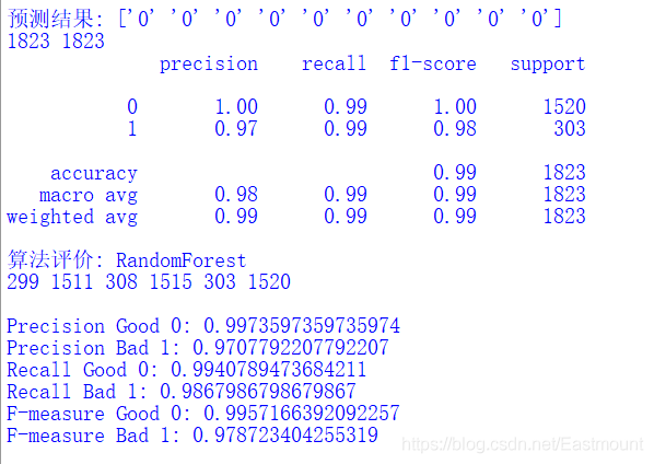
1.RandomForest
The code is as follows:
# Random forest classification method model n_estimators: number of trees in the forest
clf = RandomForestClassifier(n_estimators=20)
clf.fit(X_train, y_train)
print('Accuracy of model:{}'.format(clf.score(X_test, y_test)))
print("\n")
pre = clf.predict(X_test)
print('Prediction results:', pre[:10])
print(len(pre), len(y_test))
print(classification_report(y_test, pre))
classification_pj("RandomForest", y_test, pre)
print("\n")
Output results:
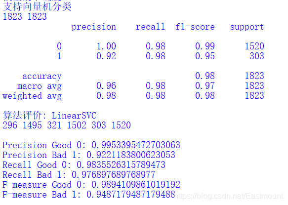
2.SVM
The code is as follows:
# SVM classification method model
SVM = svm.LinearSVC() #Support vector machine classifier LinearSVC
SVM.fit(X_train, y_train)
print('Accuracy of model:{}'.format(SVM.score(X_test, y_test)))
pre = SVM.predict(X_test)
print("Support vector machine classification")
print(len(pre), len(y_test))
print(classification_report(y_test, pre))
classification_pj("LinearSVC", y_test, pre)
print("\n")
Output results:
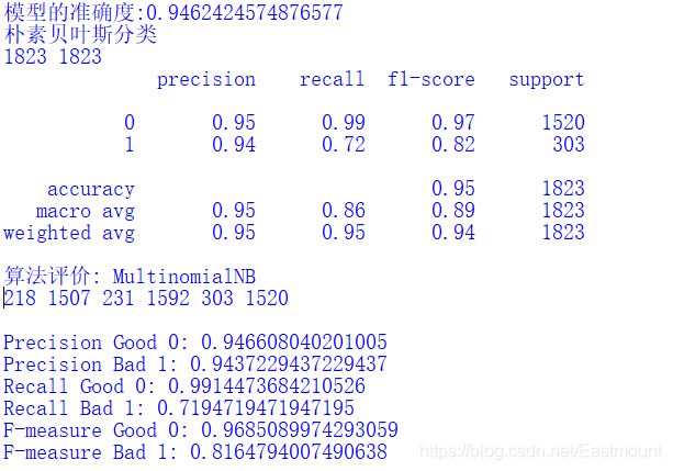
3. Naive Bayes
The code is as follows:
#naive bayesian model
nb = MultinomialNB()
nb.fit(X_train, y_train)
print('Accuracy of model:{}'.format(nb.score(X_test, y_test)))
pre = nb.predict(X_test)
print("naive bayesian classification ")
print(len(pre), len(y_test))
print(classification_report(y_test, pre))
classification_pj("MultinomialNB", y_test, pre)
print("\n")
Output results:
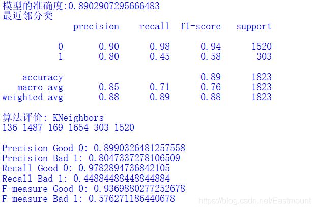
4.KNN
The accuracy of the algorithm is not high, and the execution time is long. It is not recommended to be used for text analysis. In some cases, the algorithm comparison is OK. The core code is as follows:
#Nearest neighbor algorithm
knn = neighbors.KNeighborsClassifier(n_neighbors=7)
knn.fit(X_train, y_train)
print('Accuracy of model:{}'.format(knn.score(X_test, y_test)))
pre = knn.predict(X_test)
print("Nearest neighbor classification")
print(classification_report(y_test, pre))
classification_pj("KNeighbors", y_test, pre)
print("\n")
Output results:
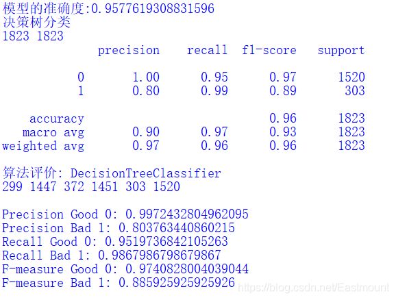
5. Decision tree
The code is as follows:
#Decision tree algorithm
dtc = DecisionTreeClassifier()
dtc.fit(X_train, y_train)
print('Accuracy of model:{}'.format(dtc.score(X_test, y_test)))
pre = dtc.predict(X_test)
print("Decision tree classification")
print(len(pre), len(y_test))
print(classification_report(y_test, pre))
classification_pj("DecisionTreeClassifier", y_test, pre)
print("\n")
Output results:
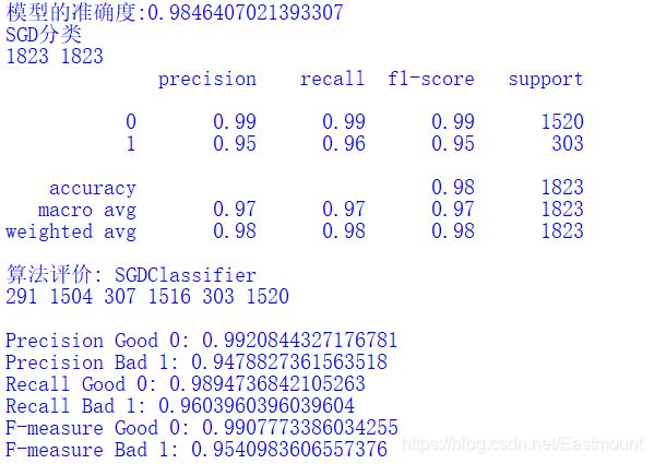
6.SGD
The code is as follows:
#SGD classification model
from sklearn.linear_model.stochastic_gradient import SGDClassifier
sgd = SGDClassifier()
sgd.fit(X_train, y_train)
print('Accuracy of model:{}'.format(sgd.score(X_test, y_test)))
pre = sgd.predict(X_test)
print("SGD classification")
print(len(pre), len(y_test))
print(classification_report(y_test, pre))
classification_pj("SGDClassifier", y_test, pre)
print("\n")
Output results:
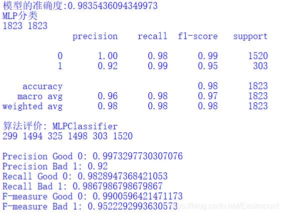
7.MLP
The algorithm is slow, and the core code is as follows:
#MLP classification model
from sklearn.neural_network.multilayer_perceptron import MLPClassifier
mlp = MLPClassifier()
mlp.fit(X_train, y_train)
print('Accuracy of model:{}'.format(mlp.score(X_test, y_test)))
pre = mlp.predict(X_test)
print("MLP classification")
print(len(pre), len(y_test))
print(classification_report(y_test, pre))
classification_pj("MLPClassifier", y_test, pre)
print("\n")
Output results:
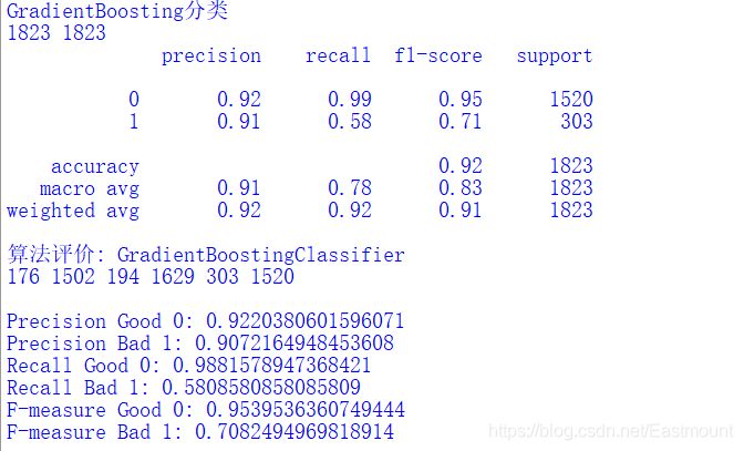
8.GradientBoosting
The algorithm is slow, and the code is as follows:
#GradientBoosting classification model
from sklearn.ensemble import GradientBoostingClassifier
gb = GradientBoostingClassifier()
gb.fit(X_train, y_train)
print('Accuracy of model:{}'.format(gb.score(X_test, y_test)))
pre = gb.predict(X_test)
print("GradientBoosting classification")
print(len(pre), len(y_test))
print(classification_report(y_test, pre))
classification_pj("GradientBoostingClassifier", y_test, pre)
print("\n")
Output results:
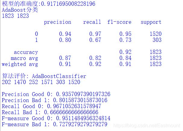
9.AdaBoost
The code is as follows:
#AdaBoost classification model
from sklearn.ensemble import AdaBoostClassifier
AdaBoost = AdaBoostClassifier()
AdaBoost.fit(X_train, y_train)
print('Accuracy of model:{}'.format(AdaBoost.score(X_test, y_test)))
pre = AdaBoost.predict(X_test)
print("AdaBoost classification")
print(len(pre), len(y_test))
print(classification_report(y_test, pre))
classification_pj("AdaBoostClassifier", y_test, pre)
print("\n")
Output results:
Click focus to learn about Huawei cloud's new technologies for the first time~