Programming environment: Python 3 seven Game question link

In today's society, housing rent is comprehensively determined by decoration, location, house type pattern, transportation convenience, market supply and demand and other factors. For the relatively traditional industry of housing rental, serious information asymmetry has always existed. On the one hand, the landlord does not understand the real market price of rental housing, so he can only bear the pain to empty the high rent housing; On the other hand, tenants can not find high cost-effective houses to meet their needs, which leads to a great waste of rental resources.

The big data competition in this computer skills competition will provide real rental market data after desensitization based on the pain points of the rental market. Players need to use the historical data with monthly rent label to establish a model to realize the prediction of monthly housing rent based on basic housing information, so as to provide an objective measurement standard for the urban rental market.

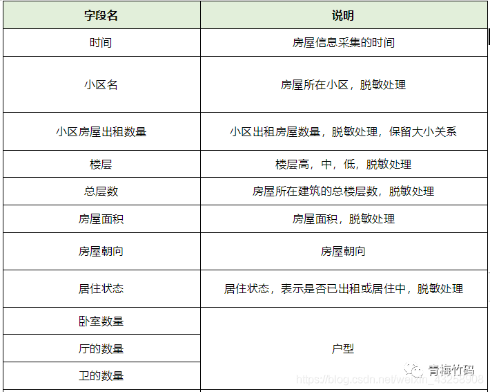
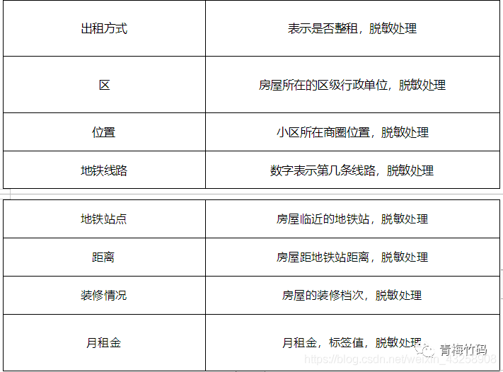
The competition data is the four-month house rental price and the basic information of the house. The official desensitized the data. Contestants need to use the house information in the data set and the monthly rent training model, and use the house information in the test set to predict the monthly rent of the house in the test data set. The data set is divided into two groups: training set and test set. The training set is the data collected in the first three months, with a total of 196539 pieces. The test set is the data collected in the fourth month. Compared with the training set, the "id" field is added, which is the unique id of the house, and there is no "monthly rent" field. Other fields are the same as the training set, with a total of 56279 items. The evaluation index is RMSE (root mean square error), which is a common evaluation index of regression algorithm. The training set contains the following fields:

other

The algorithm measures the quality of the regression model by calculating the root mean square error between the predicted value and the real monthly rent. The smaller the root mean square error, the better the regression model. The root mean square error is calculated as follows:

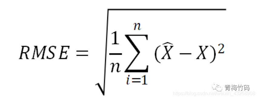
Among them, is the predicted value of the monthly rent of the house submitted by the contestant, and is the real monthly rent of the corresponding house.

This paper mainly explains from the following aspects: data cleaning, feature construction, model training and model fusion

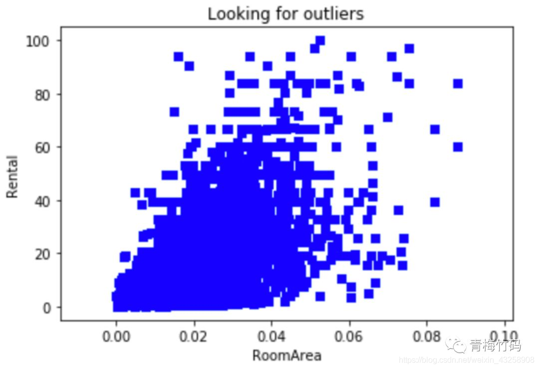
Data cleaning

The scatter diagram showing the relationship between house area and monthly rent is as follows:

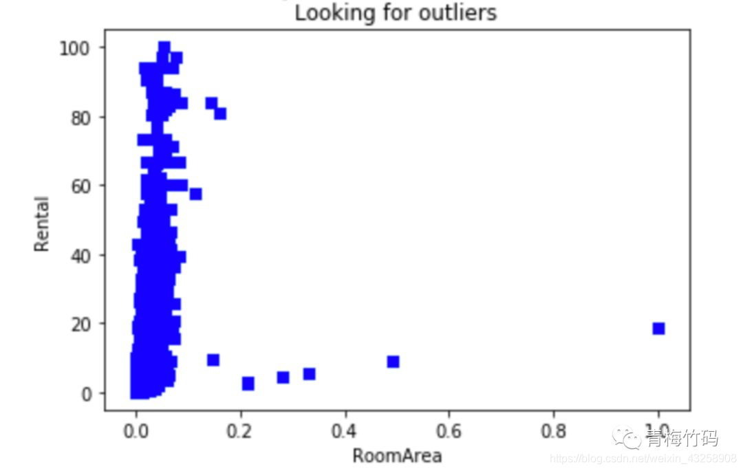
After the outliers are cleared, the scatter diagram of the relationship between house area and monthly rent is drawn as follows:

After testing, removing outliers can improve the performance of the model.

Characteristic structure

First, construct the features according to common sense, such as the total number of rooms, bedroom area, hall area, bathroom area, room relative height, etc. Then, common routines are used to construct features, such as LabelEncoder coding of category features, linear combination of multiple features, proportional features and so on.

Then the RMSE obtained from the original features is used as the baseline, and the useful structural features are selected by comparing the size of RMSE and baseline after adding new structural features.

Construct features according to common sense The so-called feature construction based on common sense is that we infer which features have strong correlation with monthly rent according to the existing knowledge.

# Total number of rooms, average area of a single room, bedroom area, hall area, bathroom area
train_df['Total rooms']=train_df['Number of bedrooms'] + train_df['Number of halls'] + train_df['Number of guards']
test_df['Total rooms']=test_df['Number of bedrooms'] + test_df['Number of halls'] + test_df['Number of guards']
train_df['Area/Room']=train_df['House area'] / (train_df['Total rooms']+1)
test_df['Area/Room']=test_df['House area'] / (test_df['Total rooms']+1)
train_df['Bedroom area']=train_df['House area']*(train_df['Number of bedrooms']/train_df['Total rooms'])
test_df['Bedroom area']=test_df['House area']*(test_df['Number of bedrooms']/test_df['Total rooms'])
train_df['Area of the hall']=train_df['House area']*(train_df['Number of halls']/train_df['Total rooms'])
test_df['Area of the hall']=test_df['House area']*(test_df['Number of halls']/test_df['Total rooms'])
train_df['Area of satellite']=train_df['House area']*(train_df['Number of guards']/train_df['Total rooms'])
test_df['Area of satellite']=test_df['House area']*(test_df['Number of guards']/test_df['Total rooms'])
# Count the number of subway stations near each community
temp = train_df.groupby('Community name')['Subway station'].count().reset_index()
temp.columns = ['Community name','Number of subway stations']
train_df = train_df.merge(temp, how = 'left',on = 'Community name')
test_df = test_df.merge(temp, how = 'left',on = 'Community name')

According to the structural characteristics of routine

Encode categorical or discrete data (e.g LabelEncoder Coding one-hot Coding), proportional features, linear combination of features, etc.

# LabelEncoder the orientation of the house
lb_encoder=LabelEncoder()
lb_encoder.fit(train_df.loc[:,'House orientation'].append(test_df.loc[:,'House orientation']))
train_df.loc[:,'House orientation']=lb_encoder.transform(train_df.loc[:,'House orientation'])
test_df.loc[:,'House orientation']=lb_encoder.transform(test_df.loc[:,'House orientation'])
# Structural 'relative height' feature
train_df['Relative height']=train_df['floor'] / (train_df['Total floor'] + 1)
test_df['Relative height']=test_df['floor'] / (test_df['Total floor'] + 1)
# Characteristics of structure (relative height * bedroom area)
train_df['PerFloorBedroomArea'] = train_df['Relative height'] * train_df['Bedroom area']
test_df['PerFloorBedroomArea'] = test_df['Relative height'] * test_df['Bedroom area']
# You can also try other features....

model training

XGBoost and LightGBM models are used for training. The characteristics used by the two models are basically the same. Finally, XGBoost single-mode online score is 1.84 and LightGBM single-mode online score is 1.88.

# xgb model parameters
xgb.XGBRegressor(max_depth=8, # The greater the depth of the construction tree, the easier it is to over fit
                 n_estimators=3880, # Optimal number of iterations
                 learning_rate=0.1, # Learning rate
                 n_jobs=-1) # Start all cpu cores

# lbg model parameters
lgb.LGBMRegressor(objective='regression',  # Objective function: Regression
                  num_leaves=900, # Number of leaf nodes
                  learning_rate=0.1, # Learning rate
                  n_estimators=3141, # Optimal iteration rounds
                  bagging_fraction=0.7, # Sample sampling ratio for tree building
                  feature_fraction=0.6, # Feature selection scale of tree building
                  reg_alpha=0.3, # L1 regularization
                  reg_lambda=0.3, # L2 regularization
                  min_data_in_leaf=18,
                  min_sum_hessian_in_leaf=0.001)

Model fusion

The weighted fusion of XGBoost and LightGBM models is adopted here. The performance of the model is improved by continuously debugging the proportion of the two models.

# -*- coding: utf-8 -*-
import pandas as pd
lgb_df = pd.read_csv("./result/lgb.csv")
xgb_df = pd.read_csv("./result/xgb.csv")
res = pd.DataFrame()
res['id'] = lgb_df['id']
# The proportion is calculated according to the online score
# 0.62/0.38 1.82066
# 0.65/0.35 1.82041
# 0.66/0.34 1.82039
# 0.67/0.33 down
res['price'] = lgb_df['price'] * 0.34 + xgb_df['price'] * 0.66
res.to_csv('./result/new.csv', index=False)

Finally, the online score after model fusion is 1.82. It can be seen that model fusion can improve the prediction effect of the model.

summary

Model training will only improve the performance of the model to a certain extent, and Feature Engineering determines the upper limit of the model. Mining features with strong correlation with the target value is the key to the victory.

When dealing with variables, the tree based algorithm is not measured based on vector space. The value is only a category symbol, that is, there is no partial order relationship, so it can not be coded alone.

The tree based algorithm does not need feature normalization.

Tree based algorithms are not good at capturing the correlation between different features.

Both LightGBM and XGBoost can learn NaN as part of the data, so they can not deal with missing values.

Part of the training set given by the topic is used as the training effect after the test set, but not all the training sets are used as the online performance effect of training.