1, Overall structure
All neurons in the adjacent layer of neural network are connected, which is called full connection. Previously, the full connection was realized with the affinity layer.
for instance
Fully connected neural network structure:

Structure of convolutional neural network CNN:

The Conv convolution layer and Pooling layer are added, and the previous affine relu connection is replaced by Conv relu Pooling connection.
In CNN, the layer close to the output uses the previous affine relu combination, and the last output layer uses the previous affine softmax combination, which is a common CNN structure.
2, Convolution layer
The problem of fully connected neural network is that the shape of data is ignored and the three-dimensional image is input, but when input to the fully connected layer, the three-dimensional needs to be pulled into one-dimensional, which leads to the neglect of the spatial information contained in the shape, that is, fully connected and unable to use the information related to the shape.
In order to solve this problem, the data transmitted to each layer is shaped data, such as three-dimensional data.
The convolution layer performs convolution operation, just like the filtering of image processing.
For the input data, the convolution operation slides the window of the filter at a certain interval, multiplies and sums the filter elements at each position and the corresponding input elements, and carries out the so-called product accumulation operation.
In the fully connected neural network, the parameters include weight and bias.
In CNN, the number in the filter is a parameter, and the bias of the data in the filter is also a parameter. To learn the data through CNN network, find these parameters, so as to achieve excellent learning effect.
Sometimes filling is required before convolution processing, that is, filling fixed data around the input data. Filling is mainly to adjust the size of the output. When the (3,3) filter is applied to the input data of (4,4), the output is (2,2), and the output is reduced by two elements than the input, resulting in a problem. If the output is reduced every time the convolution operation is performed, the output cannot be convoluted at a certain time, and the network cannot be transmitted. If the filling amplitude of this example is 1, the convolution operation output is also (4,4), and the convolution operation can transfer data to the next layer while keeping the space size unchanged.
Increase the stride, the output size will become smaller, and increase the fill output size will become larger.
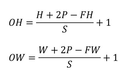
Suppose the input size is (H,W), the filter size is (FH,FW), the output size is (OH,OW), the filling is P and the step is S.
There is the following formula.

Convolution of multidimensional data:
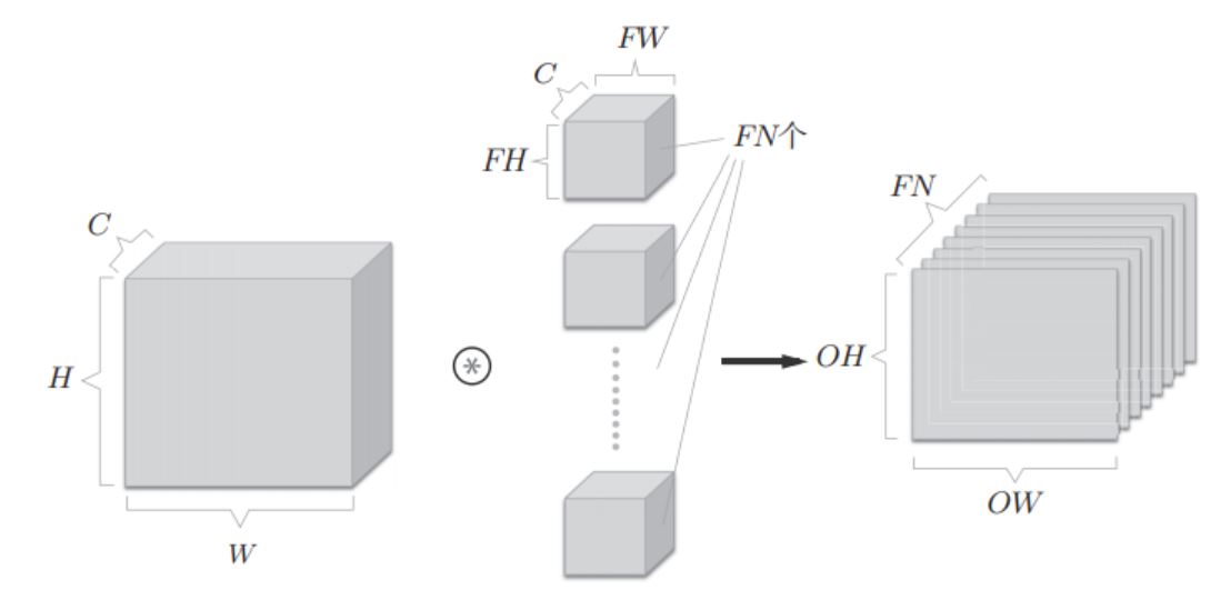
Data shape with channel number C, height H and length W, (C,H,W)
The number of filter channels is C, the height is FH, and the length is FW, (C,FH,FW)
After convolution, a characteristic graph is output. It can be understood that a small block moves in a large block. Because the C of the large block is the same as that of the small block, it is two-dimensional after convolution.

If you want to have multiple convolution operations on the channel, you need to use multiple filters, as shown in the figure below. The output will be transmitted to the next layer in the form of blocks.

If you increase the offset, as shown in the following figure: small box, that is, FN offset values.

If batch processing is added, that is, N data are processed at one time, the data saving dimension of each layer will increase by one dimension, as shown in the following figure.

3, Pool layer
Pooling is a spatial operation that reduces the height and rectangle upward. The Max pool layer obtains the maximum value of the target area, and then puts the maximum value into one of the elements of the output data. The pool layer has no parameters to learn, and the number of channels does not change. Pooling is robust to small deviation of input data, that is, when there is a small deviation of input data, the pooling layer returns the same output result (when there is no small deviation of input data).
4, python implements convolution layer and pooling layer
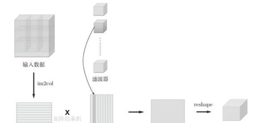
For convolution, im2col this function can expand the small blocks of large blocks into one line, so it can perform matrix product operation with the small blocks of the filter, as shown in the figure below.

For pooling, im2col can still be expanded in this way, that is, the small squares inside the large square can be expanded into a row, and the figure will not be displayed here.
im2col implementation code:
def im2col(input_data, filter_h, filter_w, stride=1, pad=0):
    """

    Parameters
    ----------
    input_data : from(Data volume, passageway, high, long)4-dimensional array of input data
    filter_h : Filter high
    filter_w : Filter length
    stride : stride
    pad : fill

    Returns
    -------
    col : 2 Dimension group
    """
    N, C, H, W = input_data.shape
    out_h = (H + 2*pad - filter_h)//stride + 1
    out_w = (W + 2*pad - filter_w)//stride + 1

    img = np.pad(input_data, [(0,0), (0,0), (pad, pad), (pad, pad)], 'constant')
    col = np.zeros((N, C, filter_h, filter_w, out_h, out_w))

    for y in range(filter_h):
        y_max = y + stride*out_h
        for x in range(filter_w):
            x_max = x + stride*out_w
            col[:, :, y, x, :, :] = img[:, :, y:y_max:stride, x:x_max:stride]

    col = col.transpose(0, 4, 5, 1, 2, 3).reshape(N*out_h*out_w, -1)
    return col
During back propagation, im2col inverse processing is performed, using the col2im function.
def col2im(col, input_shape, filter_h, filter_w, stride=1, pad=0):
    """

    Parameters
    ----------
    col :
    input_shape : Shape of input data (example:(10, 1, 28, 28))
    filter_h :
    filter_w
    stride
    pad

    Returns
    -------

    """
    N, C, H, W = input_shape
    out_h = (H + 2*pad - filter_h)//stride + 1
    out_w = (W + 2*pad - filter_w)//stride + 1
    col = col.reshape(N, out_h, out_w, C, filter_h, filter_w).transpose(0, 3, 4, 5, 1, 2)

    img = np.zeros((N, C, H + 2*pad + stride - 1, W + 2*pad + stride - 1))
    for y in range(filter_h):
        y_max = y + stride*out_h
        for x in range(filter_w):
            x_max = x + stride*out_w
            img[:, :, y:y_max:stride, x:x_max:stride] += col[:, :, y, x, :, :]

    return img[:, :, pad:H + pad, pad:W + pad]
Implementation code of convolution layer and pooling layer:
class Convolution:
    def __init__(self, W, b, stride=1, pad=0):
        self.W = W
        self.b = b
        self.stride = stride
        self.pad = pad

        # Intermediate data (used in backward)
        self.x = None
        self.col = None
        self.col_W = None

        # Gradient of weight and bias parameters
        self.dW = None
        self.db = None

    def forward(self, x):
        FN, C, FH, FW = self.W.shape
        N, C, H, W = x.shape
        out_h = 1 + int((H + 2*self.pad - FH) / self.stride)
        out_w = 1 + int((W + 2*self.pad - FW) / self.stride)

        col = im2col(x, FH, FW, self.stride, self.pad)
        col_W = self.W.reshape(FN, -1).T

        out = np.dot(col, col_W) + self.b
        out = out.reshape(N, out_h, out_w, -1).transpose(0, 3, 1, 2)

        self.x = x
        self.col = col
        self.col_W = col_W

        return out

    def backward(self, dout):
        FN, C, FH, FW = self.W.shape
        dout = dout.transpose(0,2,3,1).reshape(-1, FN)

        self.db = np.sum(dout, axis=0)
        self.dW = np.dot(self.col.T, dout)
        self.dW = self.dW.transpose(1, 0).reshape(FN, C, FH, FW)

        dcol = np.dot(dout, self.col_W.T)
        dx = col2im(dcol, self.x.shape, FH, FW, self.stride, self.pad)

        return dx


class Pooling:
    def __init__(self, pool_h, pool_w, stride=1, pad=0):
        self.pool_h = pool_h
        self.pool_w = pool_w
        self.stride = stride
        self.pad = pad

        self.x = None
        self.arg_max = None

    def forward(self, x):
        N, C, H, W = x.shape
        out_h = int(1 + (H - self.pool_h) / self.stride)
        out_w = int(1 + (W - self.pool_w) / self.stride)

        col = im2col(x, self.pool_h, self.pool_w, self.stride, self.pad)
        col = col.reshape(-1, self.pool_h*self.pool_w)

        arg_max = np.argmax(col, axis=1)
        out = np.max(col, axis=1)
        out = out.reshape(N, out_h, out_w, C).transpose(0, 3, 1, 2)

        self.x = x
        self.arg_max = arg_max

        return out

    def backward(self, dout):
        dout = dout.transpose(0, 2, 3, 1)

        pool_size = self.pool_h * self.pool_w
        dmax = np.zeros((dout.size, pool_size))
        dmax[np.arange(self.arg_max.size), self.arg_max.flatten()] = dout.flatten()
        dmax = dmax.reshape(dout.shape + (pool_size,))

        dcol = dmax.reshape(dmax.shape[0] * dmax.shape[1] * dmax.shape[2], -1)
        dx = col2im(dcol, self.x.shape, self.pool_h, self.pool_w, self.stride, self.pad)

        return dx