preface
A learning channel of Python numpy Library
1, Basic index and slicing of ndarray
Like a sequence, ndarray can also perform indexing and slicing operations. The index start sequence number also starts from 0, and ndarray can be performed in different dimensions.
① Index and slice of one-dimensional array
The index of a one-dimensional array is similar to the function of a Python list
The slicing syntax format of one-dimensional array is array[index1:index2], which means an array starting from the index1 index position and ending at the index2 index (excluding index2)
ary = np.arange(10)
ary[5] #5
ary[2:7] #array([2, 3, 4, 5, 6])
② Indexing and slicing of two-dimensional arrays
When accessing a two-dimensional array by indexing a one-dimensional array, the obtained element is no longer a scalar, but a one-dimensional array.
If the index of a two-dimensional array corresponds to a one-dimensional array, the slice of a two-dimensional array is a fragment composed of a one-dimensional array.
ary2d = np.arange(1,10).reshape((3,3))
ary2d
#array([[1, 2, 3],
#       [4, 5, 6],
#       [7, 8, 9]])
ary2d[1] #array([4, 5, 6])
ary2d[1][0] #4
ary2d[0:2] #section
#array([[1, 2, 3],
#       [4, 5, 6]])
③ Indexing and slicing of multidimensional arrays
Multidimensional array indexes only need to be selected layer by layer from outside to inside
room = np.array([[[0,1,2,3],
                 [4,5,6,7],
                 [8,9,10,11]],
                 [[12,13,14,15],
                 [16,17,18,19],
                 [20,21,22,23]]])
room[0,0,0] #It can also be written as room[0][0][0]
#0
room[0][2][3] #11
room[1][1][2] #18
room[:,0,0] #array([ 0, 12])
room[0,:,:]
#array([[ 0,  1,  2,  3],
#       [ 4,  5,  6,  7],
#       [ 8,  9, 10, 11]])
room[0,1,0:4:2] #array([4, 6])
④ Boolean index
Boolean index obtains an array of elements that meet the specified conditions through Boolean operations (such as comparison operators).
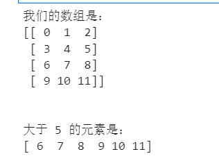
#Get elements greater than 5:
import numpy as np

x = np.array([[  0,  1,  2],[  3,  4,  5],[  6,  7,  8],[  9,  10,  11]])
print ('Our array is:')
print (x)
print ('\n')
# Now we will print out elements greater than 5
print  ('Elements greater than 5 are:')
print (x[x >  5])
The following example uses ~ (complement operator) to filter NaN.
import numpy as np

a = np.array([np.nan,  1,2,np.nan,3,4,5])
print (a[~np.isnan(a)]) #Filter NAN
#[ 1.   2.   3.   4.   5.]
⑤ Fancy index
Fancy indexing refers to the use of an array of integers for indexing.
The fancy index takes the value of the index array as the subscript of an axis of the target array. For using a one-dimensional integer array as an index, if the target is a one-dimensional array, the index result is the row corresponding to the subscript; if the target is a two-dimensional array, it is the element corresponding to the position.
Unlike slicing, a fancy index always copies data into a new array.
#Integer array index
#Gets the elements at positions (0,0), (1,1), and (2,0) in the array.
import numpy as np

x = np.array([[1,  2],  [3,  4],  [5,  6]])
y = x[[0,1,2],  [0,1,0]]
print (y)
#[1 4 5]
#1. Pass in sequential index array
x=np.arange(32).reshape((8,4))
print (x[[4,2,1,7]])
#[[16 17 18 19]
# [ 8  9 10 11]
#[ 4  5  6  7]
#[28 29 30 31]]
#2. Pass in inverted index array
x=np.arange(32).reshape((8,4))
print (x[[-4,-2,-1,-7]])
#[[16 17 18 19]
# [24 25 26 27]
# [28 29 30 31]
# [ 4  5  6  7]]
#3. Pass in multiple index arrays (to use np.ix_)
x=np.arange(32).reshape((8,4))
print (x[np.ix_([1,5,7,2],[0,3,1,2])]) #Output a 4 * 4 matrix
#[[ 4  7  5  6]
# [20 23 21 22]
# [28 31 29 30]
# [ 8 11  9 10]]
np.xi_ If two lists are input, the first list stores the row labels of the elements to be extracted, and the second list stores the column labels of the elements to be extracted. Each element in the first list will traverse each value in the second list to form a row element of the new matrix.
2, Morphological transformation operation of ndarray
① reshape() function
The reshape(shape) function changes the shape of the array and returns an array of the specified shape.
import numpy as np
Array1 = np.arange(12)
Array2 = Array1.reshape((2,6))
Array2
#array([[ 0,  1,  2,  3,  4,  5],
#       [ 6,  7,  8,  9, 10, 11]])
Array3 = Array1.reshape((2,2,3))
Array3
#array([[[ 0,  1,  2],
#        [ 3,  4,  5]],

#       [[ 6,  7,  8],
#        [ 9, 10, 11]]])
Array1 #array([ 0,  1,  2,  3,  4,  5,  6,  7,  8,  9, 10, 11])
#The reshape() function does not change the original array
② resize() function
The resize(new_shape) function directly changes the original array into an array specifying a new shape and returns a null value.
Array1.resize((3,4))
Array1 #The resize() function changes the original array
#array([[ 0,  1,  2,  3],
#       [ 4,  5,  6,  7],
#       [ 8,  9, 10, 11]])
③ Transfer() function
The transfer (* axes) function can transpose the array by axis, also known as dimension transformation, and return the transposed new array.
import numpy as np
Array1 = np.arange(12)
Array1 #array([ 0,  1,  2,  3,  4,  5,  6,  7,  8,  9, 10, 11])
Array1.resize((3,4))
Array1
#array([[ 0,  1,  2,  3],
#       [ 4,  5,  6,  7],
#       [ 8,  9, 10, 11]])
Array4 = Array1.transpose() #Transpose from (3,4) to (4,3) axis 0 and axis 1 are interchangeable
Array4
#array([[ 0,  4,  8],
#       [ 1,  5,  9],
#       [ 2,  6, 10],
#       [ 3,  7, 11]])
Array5 = np.arange(24).reshape((2,3,4)).transpose((0,2,1)) #Row column transpose
#array([[[ 0,  4,  8],
#        [ 1,  5,  9],
#        [ 2,  6, 10],
#        [ 3,  7, 11]],

#       [[12, 16, 20],
#       [13, 17, 21],
#       [14, 18, 22],
#       [15, 19, 23]]])
Array5.transpose() #The order of the fully transposed axis changes to (2,1,0) 2 axis 1 axis 0 axis
#array([[[ 0, 12],
#        [ 1, 13],
#        [ 2, 14],
#        [ 3, 15]],

#      [[ 4, 16],
#       [ 5, 17],
#       [ 6, 18],
#       [ 7, 19]],

#     [[ 8, 20],
#      [ 9, 21],
#       [10, 22],
#        [11, 23]]])
④ flatten() function
The flatten() function is used to flatten the array, that is, convert the high-dimensional array into a one-dimensional array. This function returns the new one-dimensional array.
Array6 = np.arange(6).reshape((2,3))
Array6
#array([[0, 1, 2],
#       [3, 4, 5]])
Array7 = Array6.flatten()
Array7
#array([0, 1, 2, 3, 4, 5])
3, Common statistical methods of ndarray
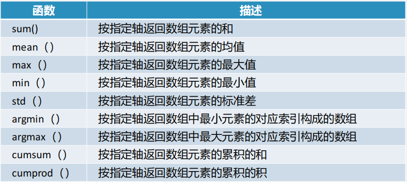
Array6 = np.arange(6).reshape((2,3))
#array([[0, 1, 2],
#        [3, 4, 5]]
Array6.sum() #Sum all elements in the array
# 15
Array6.sum(axis=0)
#The array is summed in the direction of 0 axis, that is, by column, and forms a new array to return
#array([3, 5, 7])
Array6.sum(axis=1)
#The array is summed in the direction of axis 1, that is, it is summed in rows, and forms a new array to return
#array([ 3, 12])
Array6.max()
#5
Array6.max(axis=0)
#array([3, 4, 5])
Array6.max(axis=1)
#array([2, 5])
Array6.cumsum(axis=0)
#The array is accumulated and summed in the direction of axis 0, that is, the current row is the sum of all the previous row elements
#array([[0, 1, 2],
#       [3, 5, 7]], dtype=int32)
Array6.cumsum(axis=1)
#The array is cumulatively summed in the direction of the first axis, that is, when the front row is the sum of all the previous column elements
#array([[ 0,  1,  3],
#       [ 3,  7, 12]], dtype=int32)