preface

  I finally finished my final homework, I can't catch me (No. last time I talked about solving linear equations by LU decomposition, but sometimes when the equations are incompatible, the conventional method will fail. At this time, we can use the least square method. Of course, for matrix fitting, we can directly calculate the least square approximation solution by using the M-P generalized inverse introduced later!

Text start~ CSDN (゜ - ゜) cheers

Knowledge points

  completely ignorant children's shoes can read relevant knowledge of linear algebra or matri x theory~

1. For the matrix inverse in the conventional sense, we have A B = B A = I AB=BA=I AB=BA=I form, where A is an n-order reversible matrix and B is its inverse matrix, which is written as A − 1 = B A^{-1}=B A−1=B.

2. If matrix A satisfies the condition A H A = A A H A^{H}A=AA^{H} AHA=AAH, then A is A normal matrix with r a n k ( A ) = r a n k ( A H A ) = r a n k ( A A H ) rank(A)=rank(A^{H}A)=rank(AA^{H}) rank(A)=rank(AHA)=rank(AAH). The necessary and sufficient condition for a normal matrix is that a has n linearly independent eigenvectors and they form a space C n C^n Standard orthogonal basis of Cn. If at this time A H A A^{H}A AHA is a positive definite matrix, i.e r a n k ( A H A ) = n rank(A^{H}A)=n rank(AHA)=n, then A H A A^{H}A AHA is reversible and corresponds to n non-zero eigenvalues.

3. If present A ∈ C m × n , B ∈ C n × m A \in C^{m \times n}, B \in C^{n \times m} A∈Cm × n,B∈Cn × m. Make B A = I n BA=I_n BA=In​. Then A is said to be left invertible and B is A left inverse matrix of A, denoted as A L − 1 A_L^{-1} AL−1​. In the textbook of matrix theory (Yang Ming, Liu Xianzhong), it is proved that for left reversible matrix A, it has the property of full rank, that is r a n k ( A ) = n rank(A)=n rank(A)=n, then it can be known from knowledge point 1, A H A A^{H}A AHA is reversible, where A has A left inverse matrix ( A H A ) − 1 A H (A^{H}A)^{-1}A^{H} (AHA)−1AH.

4. Similarly, if it exists C ∈ C n × m C \in C^{n \times m} C∈Cn × m. Make A C = I m AC=I_m AC=Im, then C is A right inverse matrix of A, written as A R − 1 A_R^{-1} AR−1​. At this time, it can be proved that A is row full rank and A has A right inverse matrix A H ( A A H ) − 1 A^{H}(AA^{H})^{-1} AH(AAH)−1.

5. On the basis of left inverse and right inverse, a minus sign generalized inverse is proposed A G A = A AGA=A AGA=A, it can be proved that the left inverse and the right inverse automatically meet the definition of minus inverse.

6. Based on the minus sign inverse, Moore and Penrose proposed the generalized plus sign inverse, which satisfies:
   (1) A G A = A AGA=A AGA=A
   (2) G A G = G GAG=G GAG=G
   (3) ( A G ) H = A G (AG)^H=AG (AG)H=AG
   (4) ( G A ) H = G A (GA)^H=GA (GA)H=GA
   Note that the generalized plus sign inverse G is A + A^+ A+.

   If matrix A is full rank, its plus sign inverse is ( A H A ) − 1 A H (A^{H}A)^{-1}A^{H} (AHA)−1AH；
   If matrix A is row full rank, its plus sign inverse is A H ( A A H ) − 1 A^{H}(AA^{H})^{-1} AH(AAH)−1.

7. Combined with what we mentioned earlier Full rank decomposition , it can be proved that the following conclusions can be obtained for any matrix A ∈ C m × n A \in C^{m \times n} A∈Cm × n has generalized plus sign inverse, let r a n k ( A ) = r rank(A)=r rank(A)=r, A full rank decomposition of A is A = B C ， B ∈ C m × r , C ∈ C r × m A=BC，B \in C^{m \times r}, C \in C^{r \times m} A=BC，B∈Cm × r,C∈Cr × m. Then there
   A + = C R − 1 B L − 1 = C H ( C C H ) − 1 ( B H B ) − 1 B H A^{+} = C_R^{-1}B_L^{-1}=C^{H}(CC^H)^{-1}(B^HB)^{-1}B^H A+=CR−1​BL−1​=CH(CCH)−1(BHB)−1BH.

8. With the help of orthogonal projection transformation (interested uu can refer to relevant data, which is not expanded here), we can prove that for incompatible equations A x = b Ax=b Ax=b， x 0 = A + b x_0=A^+b x0 = A+b is the best least squares solution, and the meaning here is that the least squares solution is the best approximation under norm constraints.

Elementary line transformation inversion

   as can be seen from the above, in order to obtain the best least squares solution of the incompatible matrix, we need to find the generalized plus sign inverse of A, which requires the full rank decomposition of A (in fact, singular value decomposition can also be used, but I haven't filled in hhh for this pit), and then calculate the left and right inverse of the result of full rank decomposition, So the most essential operation is how to calculate the inverse of the matrix (here we can guarantee the matrix) A A H AA^{H} AAH or A H A A^{H}A AHA is reversible). The most common method, from freshman to freshman, is, of course, the inverse of elementary line transformation. The general idea (or A long sentence) is to form A matrix and identity matrix into A large matrix [ A ∣ I ] [A|I] [a ∣ I], while transforming a into a unit matrix through elementary row transformation, the matrix obtained by the unit matrix on the right under the same operation is the inverse matrix of A.

code implementation

@classmethod
def Primary_Row_Transformation_Inv(self, target, eps=1e-6, test=False):
    """Primary_Row_Transformation_Inv 

    Args:
        target ([np.darray]): [target matrix]
        eps ([float]): numerical threshold.
        test (bool, optional): [whether to show testing information]. Defaults to False.

    Returns:
        [np.darray]: [A-]
	
	Last edited: 22-01-09
    Author: Junno
    """
    assert len(np.shape(target)) == 2
    # get row and col numbers
    M, N = np.shape(target)
    assert M == N, 'This matrix is not square-like, so it can\'t use PRT to get inverse and you can use MP-inverse to calculate its general inv'
    assert self.Get_row_rank(
        target) == M, 'This matrix is not full-rank, so it can\'t use PRT to get inverse and you can use MP-inverse to calculate its general inv'
    E = np.eye(M)
    A = deepcopy(target)
    if test:
        print('original matrix:')
        print(target)

    for i in range(M):
        for j in range(i, N):
            if test:
                print('During process in row:{}, col:{}'.format(i, j))
            if sum(abs(A[i:, j])) > eps:
                # sort rows by non-zero values from small to large
                zero_index = []
                non_zero_index = []
                for k in range(i, M):
                    if abs(A[k, j]) > eps:
                        non_zero_index.append(k)
                    else:
                        zero_index.append(k)

                non_zero_index = sorted(
                    non_zero_index, key=lambda x: abs(A[x, j]))
                sort_cols = non_zero_index+zero_index
                if test:
                    print("Sort_cols index: {}".format(sort_cols))

                # E should be processed with the same operations.
                A[i:, :] = A[sort_cols, :]
                E[i:, :] = E[sort_cols, :]

                if test:
                    print('After resorting')
                    print(A)
                    print(E)

                # eliminate elements belows
                prefix = -A[i+1:, j]/A[i, j]
                temp = (np.array(prefix).reshape(-1, 1)
                        )@A[i, :].reshape((1, -1))
                A[i+1:, :] += temp

                temp = (np.array(prefix).reshape(-1, 1)
                        )@E[i, :].reshape((1, -1))
                E[i+1:, :] += temp

                if test:
                    print('After primary row transformation:')
                    print(A)
                    print(E)

                # eliminate elements above
                for k in range(i):
                    if abs(A[k, j]) > eps:
                        # be careful to using intermediate parameter
                        temp = -(A[k, j]/A[i, j])
                        A[k, :] += temp*A[i, :]
                        E[k, :] += temp*E[i, :]

                if test:
                    print('After eliminating elements above:')
                    print(A)
                    print(E)

                break

            else:
                continue
	
	# normalize the first element of each row to 1
    for m in range(M):
        if abs(A[m, m]) > eps:
            if A[m, m] != 1:
                temp = 1./A[m, m]
                A[m, :] *= temp
                E[m, :] *= temp

    return E

test example

>>> import numpy as np
>>> from Matrix_Solutions import Matrix_Solutions
>>> A=np.array([[ 1., -3.,  7.],
...        [ 2.,  4., -3.],
...        [-3.,  7.,  2.]], dtype=np.float32)

>>> inv_A=Matrix_Solutions.Primary_Row_Transformation_Inv(A)          
>>> inv_A
array([[ 0.148,  0.281, -0.097],
       [ 0.026,  0.117,  0.087],
       [ 0.133,  0.01 ,  0.051]])

>>> A@inv_A
array([[ 1., -0., -0.],
       [-0.,  1., -0.],
       [ 0.,  0.,  1.]])
>>> inv_A@A
array([[ 1.,  0., -0.],
       [ 0.,  1.,  0.],
       [-0.,  0.,  1.]])

  with the inverse tool, our various generalized inverses are natural and can be directly written into the code

@classmethod
def Left_inv(self, target):
	"""Get_Left_Inv 

    Args:
        target ([np.darray]): [target matrix]

    Returns:
        [np.darray]: [A_L]

	Last edited: 22-01-09
    Author: Junno
    """
    assert len(np.shape(target)) == 2
    # get row ans col numbers
    M, N = np.shape(target)
    assert self.Get_col_rank(target) == N
    return self.Primary_Row_Transformation_Inv(target.T@target)@target.T

@classmethod
def Right_inv(self, target):
	"""Get_Right_Inv 

    Args:
        target ([np.darray]): [target matrix]

    Returns:
        [np.darray]: [A_R]

	Last edited: 22-01-09
    Author: Junno
    """
    assert len(np.shape(target)) == 2
    # get row ans col numbers
    M, N = np.shape(target)
    assert self.Get_row_rank(target) == M
    return target.T@self.Primary_Row_Transformation_Inv(target@target.T)

@classmethod
def Moore_Penrose_General_Inv(self, target):
    """Moore_Penrose_General_Inv 

    Args:
        target ([np.darray]): [target matrix]

    Returns:
        [np.darray]: [A+]

	Last edited: 22-01-09
    Author: Junno
    """
    assert len(np.shape(target)) == 2
    # get row ans col numbers
    M, N = np.shape(target)
    B, C = self.Full_Rank_Fact(target)
    return self.Right_inv(C)@self.Left_inv(B)

test example

>>> test_m=np.array([
...     [1,0,-1,1],
...     [0,2,2,2], 
...     [-1,4,5,3]
... ]).reshape((3,4)).astype(np.float32)

>>> test_m
array([[ 1.,  0., -1.,  1.],
       [ 0.,  2.,  2.,  2.],
       [-1.,  4.,  5.,  3.]], dtype=float32)
       
>>> MPI=Matrix_Solutions.Moore_Penrose_General_Inv(test_m)
>>> MPI
array([[ 0.278,  0.111, -0.056], 
       [ 0.056,  0.056,  0.056], 
       [-0.222, -0.056,  0.111], 
       [ 0.333,  0.167,  0.   ]])
       
# AGA=A
>>> test_m@MPI@test_m
array([[ 1.,  0., -1.,  1.],
       [-0.,  2.,  2.,  2.],
       [-1.,  4.,  5.,  3.]])
       
# GAG=G       
>>> MPI@test_m@MPI
array([[ 0.278,  0.111, -0.056],
       [ 0.056,  0.056,  0.056],
       [-0.222, -0.056,  0.111],
       [ 0.333,  0.167,  0.   ]])
       
# (AG)^T=AG, that is, Ag is a symmetric matrix
>>> test_m@MPI                 
array([[ 0.833,  0.333, -0.167],
       [ 0.333,  0.333,  0.333],
       [-0.167,  0.333,  0.833]])
       
# (GA)^T=GA, that is, GA is a symmetric matrix
>>> (MPI@test_m)  
array([[ 0.333,  0.   , -0.333,  0.333],
       [ 0.   ,  0.333,  0.333,  0.333],
       [-0.333,  0.333,  0.667, -0.   ],
       [ 0.333,  0.333,  0.   ,  0.667]])

Applying: fitting data point curves

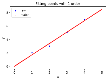
   the most common application of the least square method is to fit the curve, minimize the distance between the curve and each observation point, and obtain the corresponding relationship between x and y. Give an example in the textbook:
   with a set of experimental data, (1, 2), (2, 3), (3, 5), (4, 7), we want to use a straight line
y = β 0 + β 1 x y=\beta_0+\beta_1 x y= β 0​+ β 1 × x to fit the data points and find the best fitting line. List matrix form:
[ 1 1 1 2 1 3 1 4 ] [ β 0 β 1 ] = [ 2 3 5 7 ] \begin{bmatrix} 1 & 1 \\ 1 & 2 \\ 1 & 3 \\ 1 & 4 \end{bmatrix} \begin{bmatrix} \beta_0\\ \beta_1 \end{bmatrix}= \begin{bmatrix} 2 \\ 3 \\ 5 \\ 7 \end{bmatrix} ⎣⎢⎢⎡​1111​1234​⎦⎥⎥⎤​[β0​β1​​]=⎣⎢⎢⎡​2357​⎦⎥⎥⎤​
   let the coefficient matrix be A, then we just need to find the generalized inverse of A, then β \beta β It can be expressed as A + b A^+b A+b.
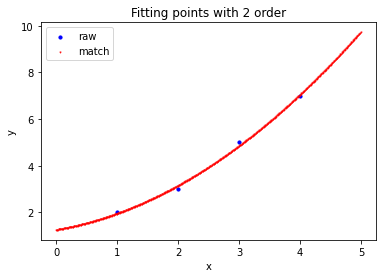
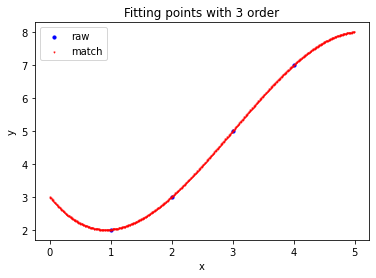
Finally, the fitting error can be determined by ∣ ∣ δ ∣ ∣ 2 = ∣ ∣ A β − b ∣ ∣ 2 ||\delta||_2=||A\beta-b||_2 ∣∣ δ ∣∣2​=∣∣A β − b ∣∣ 2. Of course, we can also use high-order fitting, so the error will be smaller, which will also be reflected in the following implementation.

code implementation

@classmethod
def Match_Points_LSM(self, ps, order):
    """Match Points using LSM and show results

    Args:
        ps ([type]): [arrays of (x,y) points]
        order ([type]): [fitting order]
	
	Last edited: 21-12-31
    Author: Junno
    """
    M, N = ps.shape[0], order+1
    A = np.zeros((M, N))
    # generate coefficient matrix A with given order
    for c in range(N):
        A[:, c] = np.power(ps[:, 0], c)
    # get MP-inv of A
    L_Inv = self.Moore_Penrose_General_Inv(A)
    # solve beta
    beta = L_Inv@ps[:, 1]

    # show results
    print('The matching line: y=', sep='', end='')
    for i in range(order+1):
        print('{:-.3f}*x^{}'.format(beta[i], i), sep='', end='')
    print('\n')

    # calculate fitting error
    error = np.linalg.norm(A@beta-ps[:, 1])
    print("Norm of Matching Error: {:.5f}".format(error))

    # prepare to show matching line
    x = np.arange(np.min(ps[:, 0])-1,
                  np.max(ps[:, 0])+1, 0.01).reshape((-1,))
    B = np.zeros((x.shape[0], N))
    for c in range(N):
        B[:, c] = np.power(x, c)
    y = B@beta

    plt.figure(0)
    fig, ax = plt.subplots()
    raw = ax.scatter(ps[:, 0], ps[:, 1], marker='o', c='blue', s=10)
    match = ax.scatter(x, y, marker='v', c='red', s=1)
    plt.legend([raw, match], ['raw', 'match'], loc='upper left')
    plt.title('Fitting points with {} order'.format(order))
    plt.xlabel('x')
    plt.ylabel('y')
    plt.show()

test example

>>> a=np.array([
...     [1,2],
...     [2,3],
...     [3,5],
...     [4,7]
... ]).reshape((-1,2)).astype(np.float32)

# First order fitting
>>> Matrix_Solutions.Match_Points_LSM(a,1)
The matching line: y=+0.000*x^0+1.700*x^1
Norm of Matching Error: 0.54772

# Second order fitting
>>> Matrix_Solutions.Match_Points_LSM(a,2) 
The matching line: y=+1.250*x^0+0.450*x^1+0.250*x^2
Norm of Matching Error: 0.22361

# Third order fitting
>>> Matrix_Solutions.Match_Points_LSM(a,3) 
The matching line: y=+3.000*x^0-2.333*x^1+1.500*x^2-0.167*x^3
Norm of Matching Error: 0.00000

summary

  today's content is here first. If you have any questions or corrections to the code, please leave a message. I will reply as soon as possible~
Not how profound the proof of principle is, it is more a tool to master this kind of problem-solving. Continue to fill the pit next time!

   Qugao may not be unknown, but it has its own bosom friends and clear words.