Logistic Regression

Advantages: low computational cost, easy to understand and implement.
Disadvantages: it is easy to under fit, and the classification accuracy may not be high.
Applicable data types: numerical data and nominal data.

Main idea: according to the existing data, the classification boundary resume regression formula is used to classify.

This is also an of the optimization algorithm.

Sigmoid function

Heaviside step function, also known as unit step function.
f ( x ) = 1 1 + e − 1 f(x)=\frac{1}{1+e^-1} f(x)=1+e−11​

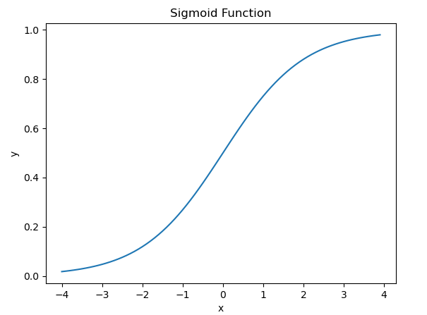
Drawing code

import numpy as np
from math import e
from matplotlib import  pyplot as plt

x=np.arange(-4,4,0.1)
y=1/(1+e**-x)
plt.xlabel('x')
plt.ylabel('y')
plt.title("Sigmoid Function")
plt.plot(x,y)
plt.show()

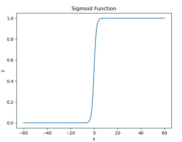
x=np.arange(-60,60,0.1)
y=1/(1+e**-x)
plt.xlabel('x')
plt.ylabel('y')
plt.title("Sigmoid Function")
plt.plot(x,y)
plt.show()

It can be seen that this is a good classification function. When the function value is greater than 0.5, the output is 1, otherwise it is 0.5

We make input Z = w T x T = w 1 x 1 + w 2 x 2 + ⋯ + w n x n Z=w^Tx^T=w_1x_1+w_2x_2+\dots+w_nx_n Z=wTxT=w1​x1​+w2​x2​+⋯+wn​xn​​​

How to get the appropriate weight vector w so that the classifier can accurately divide the data set?

Gradient rise method

The mathematical meaning of the derivative of a function is the speed of the rise and fall of the function. According to the derivative, we move along the direction of the rise of the function, and we can gradually approach the maximum point.
w : = w + α ∇ w f ( w ) w:=w+\alpha\nabla_wf(w) w:=w+α∇w​f(w)
The parameter w plus the derivative of the function at w times the learning rate α \alpha α​.​

Pseudo code

Each regression coefficient is initialized to 1
 repeat R Times:
	Calculate the gradient of the entire dataset
	use alpha*gradient Update vector of regression coefficient
 Return regression coefficient

The derivation of formulas in this book is omitted, but the author still wants to try to talk about it (a little omitted):

This involves cross entropy loss function, vectorization and maximum likelihood estimation

We want to maximize the probability that all the predicted results are correct, so the maximum likelihood estimation is useful here.

There are Sigmoid functions:
h θ ( x ) = 1 1 + e − z h_\theta(x)=\frac{1}{1+e^{-z}} hθ​(x)=1+e−z1​
Want the greatest probability.

We need to find a parameter θ \theta θ Make the discrete likelihood function:
L ( θ ) = ∏ i = 1 m ( h θ ( x ( i ) ) ) y ( i ) ( 1 − h θ ( x ( i ) ) ) 1 − y ( i ) L(\theta)=\prod_{i=1}^m(h_\theta(x^{(i)}))^{y^(i)}(1-h_\theta(x^{(i)}))^{1-y^{(i)}} L(θ)=i=1∏m​(hθ​(x(i)))y(i)(1−hθ​(x(i)))1−y(i)
Since the continuous multiplication is prone to underflow, we still use the method of increasing log.

Make the formula
l ( θ ) = l o g L ( θ ) = ∑ i = 1 m ( y ( i ) l o g h θ ( x ( i ) ) + ( 1 − y ( i ) ) l o g ( 1 − h θ ( x ( i ) ) ) ) l(\theta)=logL(\theta)=\sum_{i=1}^m(y^{(i)}logh_\theta(x^{(i)})+(1-y^{(i)})log(1-h_\theta(x^{(i)}))) l(θ)=logL(θ)=i=1∑m​(y(i)loghθ​(x(i))+(1−y(i))log(1−hθ​(x(i))))
In general, it is customary to make the function as small as possible. You can take symbols. However, this chapter uses the gradient rise method, that is, the larger the better.

This function is also called cross entropy loss function.

According to the gradient rise method, we need to find the derivative of this function, just note that this is a composite function.

Finally, we can get:
∂ θ j J ( θ ) = ( y − h θ ( x ) ) x j \frac{\partial}{\theta_j}J(\theta)=(y-h_\theta(x))x_j θj​∂​J(θ)=(y−hθ​(x))xj​

Gradient rise iteration formula:
θ j : = θ j + α ∑ i = 1 m ( y ( i ) − h θ ( x ( i ) ) ) x j ( i ) \theta_j:=\theta_j+\alpha\sum_{i=1}^m(y^{(i)}-h_\theta(x^{(i)}))x_j^{(i)} θj​:=θj​+αi=1∑m​(y(i)−hθ​(x(i)))xj(i)​
In order to use the matrix operation to accelerate the band, the formula needs to be vectorized:
θ : = θ + α X T ( y − g ( x θ ) ) \theta:=\theta+\alpha X^T(y-g(x_\theta)) θ:=θ+αXT(y−g(xθ​))
This also corresponds to the following in the code:

weights = weights + alpha * dataMatrix.transpose()* error

Improved gradient rise algorithm:

• The gradient rise algorithm needs to traverse the whole data set every time it updates the coefficients. It can update the regression coefficients by using only one sample point at a time through random gradient rise.
• Adjust the alpha so that the alpha decreases with the number of iterations, but will not be zero, which is the same as the furnace temperature in simulated annealing.
• Randomly select sample points to update the regression coefficient.

logRegress.py

'''
Created on Oct 27, 2010
Logistic Regression Working Module
@author: Peter
'''
from numpy import *

def loadDataSet():
    dataMat = []; labelMat = []
    fr = open('testSet.txt')
    for line in fr.readlines():
        lineArr = line.strip().split()
        dataMat.append([1.0, float(lineArr[0]), float(lineArr[1])])
        labelMat.append(int(lineArr[2]))
    return dataMat,labelMat

def sigmoid(inX):
    return 1.0/(1+exp(-inX))

def gradAscent(dataMatIn, classLabels):
    dataMatrix = mat(dataMatIn)             #convert to NumPy matrix
    labelMat = mat(classLabels).transpose() #convert to NumPy matrix
    m,n = shape(dataMatrix)
    alpha = 0.001
    maxCycles = 500
    weights = ones((n,1))
    for k in range(maxCycles):              #heavy on matrix operations
        h = sigmoid(dataMatrix*weights)     #matrix mult
        error = (labelMat - h)              #vector subtraction
        weights = weights + alpha * dataMatrix.transpose()* error #matrix mult
    return weights

def plotBestFit(weights):
    import matplotlib.pyplot as plt
    dataMat,labelMat=loadDataSet()
    dataArr = array(dataMat)
    n = shape(dataArr)[0] 
    xcord1 = []; ycord1 = []
    xcord2 = []; ycord2 = []
    for i in range(n):
        if int(labelMat[i])== 1:
            xcord1.append(dataArr[i,1]); ycord1.append(dataArr[i,2])
        else:
            xcord2.append(dataArr[i,1]); ycord2.append(dataArr[i,2])
    fig = plt.figure()
    ax = fig.add_subplot(111)
    ax.scatter(xcord1, ycord1, s=30, c='red', marker='s')
    ax.scatter(xcord2, ycord2, s=30, c='green')
    x = arange(-3.0, 3.0, 0.1)
    y = (-weights[0]-weights[1]*x)/weights[2]
    ax.plot(x, y)
    plt.xlabel('X1'); plt.ylabel('X2');
    plt.show()

def stocGradAscent0(dataMatrix, classLabels):
    m,n = shape(dataMatrix)
    alpha = 0.01
    weights = ones(n)   #initialize to all ones
    for i in range(m):
        h = sigmoid(sum(dataMatrix[i]*weights))
        error = classLabels[i] - h
        weights = weights + alpha * error * dataMatrix[i]
    return weights

def stocGradAscent1(dataMatrix, classLabels, numIter=150):
    m,n = shape(dataMatrix)
    weights = ones(n)   #initialize to all ones
    for j in range(numIter):
        dataIndex = range(m)
        for i in range(m):
            alpha = 4/(1.0+j+i)+0.0001    #apha decreases with iteration, does not 
            randIndex = int(random.uniform(0,len(dataIndex)))#go to 0 because of the constant
            h = sigmoid(sum(dataMatrix[randIndex]*weights))
            error = classLabels[randIndex] - h
            weights = weights + alpha * error * dataMatrix[randIndex]
            del(dataIndex[randIndex])
    return weights

def classifyVector(inX, weights):
    prob = sigmoid(sum(inX*weights))
    if prob > 0.5: return 1.0
    else: return 0.0

def colicTest():
    frTrain = open('horseColicTraining.txt'); frTest = open('horseColicTest.txt')
    trainingSet = []; trainingLabels = []
    for line in frTrain.readlines():
        currLine = line.strip().split('\t')
        lineArr =[]
        for i in range(21):
            lineArr.append(float(currLine[i]))
        trainingSet.append(lineArr)
        trainingLabels.append(float(currLine[21]))
    trainWeights = stocGradAscent1(array(trainingSet), trainingLabels, 1000)
    errorCount = 0; numTestVec = 0.0
    for line in frTest.readlines():
        numTestVec += 1.0
        currLine = line.strip().split('\t')
        lineArr =[]
        for i in range(21):
            lineArr.append(float(currLine[i]))
        if int(classifyVector(array(lineArr), trainWeights))!= int(currLine[21]):
            errorCount += 1
    errorRate = (float(errorCount)/numTestVec)
    print ("the error rate of this test is: %f" % errorRate)
    return errorRate

def multiTest():
    numTests = 10; errorSum=0.0
    for k in range(numTests):
        errorSum += colicTest()
    print ("after %d iterations the average error rate is: %f" % (numTests, errorSum/float(numTests)))
        

Conclusion:

• Starting from this chapter, the three disciplines of line generation, advanced mathematics and probability theory have been applied. Learning mathematics is really important and we must use a solid foundation.
• The proportion of these steps is also increasing.
• Since I studied the model in my freshman year, I didn't study the example.